Dislocation and disclination densities in experimentally deformed polycrystalline olivine

We report a comprehensive data set characterizing and quantifying the geometrically necessary dislocation (GND) density in the crystallographic frame (${\mathit{\rho }}_{\mathit{\alpha }}^{\mathrm{c}}$) and disclination density (ρ_θ) in fine-grained polycrystalline olivine deformed in uniaxial compression or torsion, at 1000 and 1200 ^∘C, under a confining pressure of 300 MPa. Finite strains range from 0.11 up to 8.6 %, and stresses reach up to 1073 MPa. The data set is a selection of 19 electron backscatter diffraction maps acquired with conventional angular resolution (0.5^∘) but at high spatial resolution (step size ranging between 0.05 and 0.1 µm). Thanks to analytical improvement for data acquisition and treatment, notably with the use of ATEX (Analysis Tools for Electron and X-ray diffraction) software, we report the spatial distribution of both GND and disclination densities. Areas with the highest GND densities define sub-grain boundaries. The type of GND densities involved also indicates that most olivine sub-grain boundaries have a mixed character. Moreover, the strategy for visualization also permits identifying minor GND that is not well organized as sub-grain boundaries yet. A low-temperature and high-stress sample displays a higher but less organized GND density than in a sample deformed at high temperature for a similar finite strain, grain size, and identical strain rate, confirming the action of dislocation creep in these samples, even for micrometric grains (2 µm). Furthermore, disclination dipoles along grain boundaries are identified in every undeformed and deformed electron backscatter diffraction (EBSD) map, mostly at the junction of a grain boundary with a sub-grain but also along sub-grain boundaries and at sub-grain boundary tips. Nevertheless, for the range of experimental parameters investigated, there is no notable correlation of the disclination density with stress, strain, or temperature. However, a broad positive correlation between average disclination density and average GND density per grain is found, confirming their similar role as defects producing intragranular misorientation. Furthermore, a broad negative correlation between the disclination density and the grain size or perimeter is found, providing a first rule of thumb on the distribution of disclinations. Field dislocation and disclination mechanics (FDDM) of the elastic fields due to experimentally measured dislocations and disclinations (e.g., strains/rotations and stresses) provides further evidence of the interplay between both types of defects. At last, our results also support that disclinations act as a plastic deformation mechanism, by allowing rotation of a very small crystal volume.

1 Introduction

As the most abundant (> 60 % in volume) and weakest mineral phase in Earth's upper mantle, olivine, dictates the upper-mantle rheology and hence the kinematics of the upper-mantle convection and the relative rigidity of the overlaying lithospheric plate compared to the viscous asthenosphere below. Experimental deformation of olivine at temperatures relevant to the lithospheric mantle and subducting slabs (< 1200 ^∘C) and extensive studies of mantle-derived xenoliths of peridotites show that dislocation creep is the major deformation mechanism in the uppermost mantle (e.g., Hirth and Kohlstedt, 2003; Tommasi and Vauchez, 2015; Bernard et al., 2019). This mechanism of deformation is rate-controlled by dislocation motions, which are topological defects in the crystal lattice arising from translational lattice incompatibility (as measured by the Burgers vector, b). Dislocations can exhibit conservative motion (glide) in some specific planes, defining slip systems (slip direction and associated plane of glide). For a polycrystalline aggregate to undergo an arbitrary imposed homogenous deformation, five independent slip systems are required (von Mises criterion, von Mises, 1928; Hutchinson, 1977). Yet, dislocations in olivine can only glide according to three independent slip systems ([100](010), [100](001), [001](010) or [100](010), [001](010), [001](100)), which are directly constrained by the lack of glide in the [010] direction (for a brief review, see Demouchy, 2021). Therefore, an additional degree of freedom must be provided, e.g., dislocation climb or grain boundary mechanisms like grain boundary sliding or grain boundary migration. Nevertheless, (1) at temperatures < 1100 ^∘C, ionic diffusion, and thus dislocation climb in olivine, is a mechanism too slow to significantly contribute to macroscopic creep (e.g., Goetze, 1978; Evans and Goetze, 1979; Hirth and Kohlstedt, 2003; Cordier et al., 2014), and (2) dislocation-accommodated grain boundary sliding requires displacement and/or significant discontinuities at grain boundaries, including cavitation (e.g., Langdon, 2006; Gasc et al., 2019). A solution was proposed as a complementary mechanism for creep in olivine aggregates: disclinations. Disclinations are rotational topological defects arising from rotational lattice incompatibility (as expressed by the Frank rotational vector ω; de Wit, 1970), which have been mostly reported in liquid crystals (Volterra, 1907; Friedel, 1922; Frank, 1958). They were observed in polycrystalline metals (e.g., Beausir and Fressengeas, 2013; Fressengeas and Beausir, 2018) and not only in experimentally deformed polycrystalline olivine but also in natural olivine-rich rocks (Cordier et al., 2014) and were successfully modeled in forsterite (Sun et al., 2016). Historically, disclinations were thought to be too high energetically to exist in crystalline solids such as silicates (Friedel, 1922; Hirth and Lothe, 1982, p. 4; Hirth et al., 2020). In polycrystalline solids, disclinations are thought to be arranged in self-screened configurations like dipoles, thus significantly reducing the stored elastic energy in the deformed lattice (Romanov and Vladimirov, 1992; Romanov and Kolesnikova, 2009; Cordier et al., 2014; Hirth et al., 2020). As such, they can be used to describe the lattice structure when a single-valued elastic rotation field does not exist, such as for grain boundaries (Li, 1972). Disclinations might therefore prove useful in modeling high-angle grain boundaries, grain boundary ledges, deformation of nano-aggregates, and grain boundaries as sources and sinks for dislocations (e.g., Kleman and Friedel, 2008). In forsterite, Heinemann et al. (2005) has shown that only grain boundaries with disorientation angles lower than 20^∘ can be modeled with the classic dislocation-based Read–Shockley model (Read and Shockley, 1950). For high-angle boundaries, dislocation cores would overlap, invalidating this description. Consequently, a solution is to introduce periodic arrays of disclination dipoles in high-angle grain boundaries models, which has been achieved successfully in the recent years (e.g., Fressengeas et al., 2011; Upadhyay et al., 2011; Taupin et al., 2014; Sun et al., 2016, 2018). Further limitations in dislocation-based grain boundary models are induced by spatial considerations, complicating three-dimensional grain networks models (Sutton and Vitek, 1983). Disclination-based models can overcome these limitations by implementing the discontinuities of the elastic displacement (i.e., small relative rotation) of the crystal lattice along grain boundaries.

In this paper we investigate the polycrystalline olivine microstructure at high spatial resolution using conventional electron backscatter diffraction (EBSD). Specifically, we quantify geometrically necessary dislocation and disclination density in deformed polycrystalline olivine for a range of temperatures, finite strains, and stresses. We use experimentally deformed samples at high pressure from previous studies (Demouchy et al., 2012; Thieme et al., 2018), providing a new data set for finite strains up to an early steady-state stage and temperatures of 1000 and 1200 ^∘C. Additionally, we investigate the effect of acquisition setup (e.g., sample preparation and step size), data treatments such as range of disorientation, and display features such as smoothing and a user-defined scale to define the best visual display for maps of disclination density.

2 Material and methods

2.1 Experimental sample and preparation

We have selected seven deformed samples from Thieme et al. (2018) and one undeformed sample from Demouchy et al. (2012) (see Table 1). All samples are synthesized from inclusion-free single crystals of San Carlos olivine washed and pulverized in a fluid energy mill, resulting in a grain equivalent diameter of ∼ 2 µm before hot pressing and deformation. San Carlos olivines have a mean composition of (Mg_0.91Fe_0.09Ni_0.003)₂SiO₄ (e.g., Buening and Buseck, 1973; Frey and Prinz, 1978; Demouchy, 2010) and a naturally low water content (< 1 ppm wt H₂O; see e.g., Demouchy, 2010). Orthopyroxene and chromite are expected as a trace fraction only, and their presence helped buffering the silica activity and oxygen fugacity, respectively.

Table 1 Experimental parameters and mechanical results for the selected deformation experiments investigated by EBSD in this study. Original deformation curves (stress–strain) are reported in Demouchy et al. (2012) and Thieme et al. (2018). Uncertainties are up to ± 2 ^∘C for T, 20 MPa for stress, and negligible for the strain and strain rate (< 1 %).

NB: ^* denotes an EBSD map centered on a relatively large grain, thus with a low number of grains.

The fine-grained powder of San Carlos olivine was first cold-pressed in Ni capsules and subsequently sintered at 1200 ^∘C and 300 MPa (argon) for 3 h, producing dense polycrystalline cylinder ∼ 8 mm in diameter and ∼ 16 mm long. Sintered polycrystals were subsequently deformed in either uniaxial compression (Thieme et al., 2018) or torsion (Demouchy et al., 2012) in a high-pressure high-temperature deformation gas-medium apparatus (Paterson, 1990; Paterson and Olgaard, 2000). The confining pressure is 300 MPa for both types of experiments, temperature was set at 1000 ^∘C or 1200 ^∘C, and equivalent strains range from 0.11 % to 8.6 %. One sample (CMT-16-7) is a sintered but undeformed aggregated used here as a reference “starting material”. Torsion sample PI0546 contains 45 µL of deionized water added to the cold-pressed aggregate, but a very limited amount of hydrogen was embedded in the olivine lattice (see Demouchy et al., 2012, for details). The samples were previously examined by transmission electron microcopy and did not reveal the presence of cavitation induced by grain boundary sliding or stressed-induced amorphization of olivine inside the grain boundaries (Demouchy et al., 2012; Thieme et al., 2018; Samae et al., 2021). For the samples deformed in torsion, a section trough the center of the sample and perpendicular to the shear direction was cut with a low-speed saw and embedded in epoxy, while samples were cut parallel to the deformation axis for the sample deformed in axial compression. Recovered samples were then polished, including a final chemo-mechanical polish using colloidal silica (0.04 µm particles, average polishing duration of 1 h) for investigation using scanning electron microscopy (SEM) and electron backscatter diffraction (EBSD).

EBSD maps were acquired at the center of the sample deformed in axial compression, while for samples deformed in torsion, EBSD maps were acquired from three positions: (1) at the inner radius, which is at 2 mm from the outer edge; (2) at the center of the sample, which is at 1 mm from the outer edge; and (3) at outer edge. Therefore, for the torsion sample there are three areas of investigation, corresponding to three different finite shear strains, shear stress, and shear strain rates. Three maps were acquired in each area (with different map sizes and acquisition setup). The shear strain γ was calculated as γ= ($\mathit{\theta }D/\mathrm{2}l$), where θ is the angular displacement, D is the sample diameter, and l is the sample length. To allow for comparison with samples deformed in uniaxial compression, the equivalent strain rate $\dot{\mathit{\epsilon }}$ was calculated as $\dot{\mathit{ϵ}}=\dot{\mathit{\gamma }}/\sqrt{\mathrm{3}}$, where $\dot{\mathit{\gamma }}$ is the shear strain rate. Likewise, the equivalent stress σ was calculated as $\mathit{\sigma }=\mathit{\tau }\sqrt{\mathrm{3}}$, where τ is the shear stress (see Paterson and Olgaard, 2000; Demouchy et al., 2012).

2.2 Crystallographic orientation measurements and treatments

2.2.1 Acquisition

Olivine crystallographic orientation was obtained by EBSD with the CamScan X500FE CrystalProbe at Géosciences Montpellier (Université de Montpellier, France). Exposed sample surfaces were partially coated with 2–5 nm of carbon, except for a central uncoated window dedicated to EBSD mapping. The typical 1 in. epoxy plug was subsequently surrounded and partially covered by copper–carbon tape to improve conductivity and electron discharging in the sample chamber. This is a requirement for achieving high-spatial-resolution mapping on semi-conductive material such as fine-grained silicates. The beam acceleration voltage was 17–17.5 kV, the beam current was 10 nA, and the working distance was 24–25.1 mm. We used a binning of 4×4 for the EBSD camera ($\mathrm{1}/\mathrm{16}$ of the original resolution of the CCD camera) to avoid charging effect for acquisition with a fine step size (< 0.2 µm). Olivine, diopside, enstatite, and Cr-spinel were acquired during mapping. EBSD data were recorded and cleaned using the AZtecHKL and HKL Channel 5 programs and further treated with the ATEX program (Analysis Tools for Electron and X-ray diffraction; Beausir and Fundenberger, 2017) to determine dislocation and disclination densities. The theoretical framework for disclination detection and quantification is already fully detailed in Beausir and Fressengeas (2013), Cordier et al. (2014), and Fressengeas and Beausir (2018) and will not be reproduced in full here; only the basic principles are recalled below.

The noise reduction of raw data is partially performed using HKL Channel 5 Tango (Oxford Instruments) and finalized using ATEX (Beausir and Fundenberger, 2017) and can also be completed using MTEX (MATLAB toolbox; see Hielscher and Schaeben, 2008; Bachmann et al., 2010). The treatment consists of (1) removing the wild spikes defined as pixels with a misorientation of > 1^∘ to at least seven neighbors, (2) nullifying isolated non-indexed pixels and clusters of up to three non-indexed pixels, (3) filtering orientations with a Kuwahara filter with two iterations and a maximum angle of 5^∘ (this non-linear smoothing filter permits adaptive noise reduction and helps to identify sub-grain boundary domains), (4) defining internal disorientations > 10^∘ as grain boundaries (displayed in dark green) (NB: 10^∘ was chosen for consistency with Demouchy et al., 2012, and Thieme et al., 2018, while a value of 15^∘ is usually chosen for data acquired on natural peridotites displaying millimetric grain size, e.g., Demouchy et al., 2019), and (5) defining disorientations between 1 and 10^∘ as sub-grain boundaries (displayed as pale-grey lines). Since we use conventional EBSD mapping (with an average precision of 0.5^∘ on the Euler angles), we kept the same quality factor, also called the mean angular deviation (MAD < 2^∘) as in previous studies (e.g., Thieme et al., 2018). ATEX also permits displaying the MAD number variation, and average values range between 0.38 and 0.63^∘ (see Table S1 and Fig. S1 for an example of the starting material and .cft files available on Zenodo). Grain boundaries can display large values but rarely exceed 1^∘ (Fig. S1, Table S1). Finally, the densities of geometrically necessary dislocations and the densities of disclinations are solely calculated along the olivine–olivine boundaries. Potential residual enstatites or Cr-spinel grains are excluded from the data treatment.

2.2.2 Geometrically necessary dislocation densities

The density of geometrically necessary dislocations (GNDs) is not to be mistaken with the average density of mobile dislocations involved in Orowan's equation (ρ) (see Hirth and Lothe, 1982; Zoller et al., 2021). The later would be the sum of the GND and the statistically stored dislocations (SSDs), which includes loops, dipoles, or multipoles, if they are mobile and not locked into the crystal (e.g., by impurities). As the SSDs are producing a null Burgers vector and do not modify the curvature of the crystallographic lattice, they cannot be identified with the method used here, while they can be identified and quantified by transmission electron microscopy. Therefore, GND is, by definition, an imperfect proxy for total mobile (free) dislocations (that is the one in Orowan's equation), producing plastic deformation by dislocation glide. GND can only represent a fraction of the elastic energy still stored in the crystal lattice after the experiment is quenched. In this study as in others (e.g., Cordier et al., 2014; Wallis et al., 2016; Hansen et al., 2021), we will hypothesize a proportionality relationship between GND density and the total (average) mobile dislocations density accommodating the strain. While GND and SSD are unambiguously related (Mughrabi, 2001), recent study in work-hardened two-phase metals (ferrite–bainite) showed that their relationship is very complex and a function of pre-existent microstructures, increasing with finite strain (e.g., Wang et al., 2022).

Here, the Nye tensor (in µm⁻¹) is calculated and represents the density of Burgers vectors per unit surface. First the Nye tensor is calculated in the map coordinate system as follows:

$$\begin{array}{}\text{(1)}& {\mathit{\alpha }}_{ij}=b_i{t}_j,\end{array}$$

where b is the Burgers vector surface density and t is the unit line direction of the corresponding dislocation (screw dislocation when colinear, edge dislocation when orthogonal to each other). This matrix is then rotated to be placed in the crystal frame ${\mathit{\alpha }}_{ij}^{\mathrm{c}}$, denoted by a superscript “c”. For a simple cubic structure such as metals, having a unique b yields a simple relation but which remains a mere convention. The density is expressed as

$$\begin{array}{}\text{(2)}& {\mathit{\rho }}_{\mathit{\alpha }}={\displaystyle \frac{\mathrm{1}}{b}}∥{\mathit{\alpha }}_{ij}∥,\end{array}$$

with the norm of GND density defined as

$$\begin{array}{}\text{(3)}& ∥{\mathit{\alpha }}_{ij}∥=\sqrt{{\mathit{\alpha }}_{ij}\cdot {\mathit{\alpha }}_{ij}}.\end{array}$$

The Nye tensor is obtained per meter, and ρ_α is converted to per square meter (Table S1) by dividing it by the magnitude of the Burgers vector b (which is different for each slip system in olivine; e.g., if b=4.764 Å for [100] dislocation, then 1 µm⁻¹ corresponds to 2.1×10¹⁵ m⁻²). Here, we chose not to follow this convention and to divide the density by the EBSD map step size (step) to yield a proper dislocation length per volume unit (in m⁻²), which is reported in Table 2 (also given in Table S1).

$$\begin{array}{}\text{(4)}& {\mathit{\rho }}_{\mathit{\alpha }}^{\mathrm{c}}={\sum }_{i,j}{\displaystyle \frac{\left|{\mathit{\alpha }}_{ij}^{\mathrm{c}}\right|}{\mathrm{step}}}\end{array}$$

We recall that only five out of nine Nye components can be calculated from the two-dimensional EBSD map (α₁₂, α₁₃, α₂₁, α₂₃, and α₃₃); the other four are non-determined components (α₁₁, α₂₂, α₃₁, and α₃₂) of an unknown value, and here a value equal to 0 is taken for each of them for the calculation in the crystallographic framework. Subsequently, nine components in the crystallographic framework (${\mathit{\alpha }}_{ij}^{\mathrm{c}}$) can be calculated as follows:

$$\begin{array}{}\text{(5)}& {\mathit{\alpha }}_{ij}^{\mathrm{c}}={\mathbf{P}}^{\mathrm{T}}{\mathit{\alpha }}_{ij}\mathbf{P},\end{array}$$

where P is the rotation matrix and P^T is the transpose of the rotation matrix. Note that the nine resulting components have the same level of uncertainty.

Table 2 For the studied EBSD maps, we report the indexation rate after data treatment, the original step size and subsequent re-step size (italicized and bold), the number of detected grains, the average grain size, and the calculated partial GND dislocation densities. We provide the average of grain density and the median grain density for α_ij. The average of each ${\mathit{\alpha }}_{ij}^{\mathrm{c}}$ and θ_ij per grain is given in Table S1 in the Supplement. Roman numerals identify individual EBSD maps acquired for the same sample (“S” stands for small-area maps). Maps from samples deformed in torsion are taken at three different positions and hence with increasing strains. Idem number of grains: id.

^a An EBSD map centered on a relatively large grain, thus with a low number of grains. ^b Average grain sizes are calculated as the diameter of a circle with equivalent area.

2.2.3 Disclination detection, densities, and display

We recall in Fig. 1 how disclination densities are calculated from the elastic rotation field ω_e along (and not across) a grain boundary. In this example, there are two crystals with orientations given by Euler angles of (0^∘, 0^∘, 0^∘) and (45^∘, 0^∘, 0^∘), and a sub-grain (in turquoise in Fig. 1 for grain 1) is inserted into the top grain with a tilt disorientation of 3^∘ around the axis e₃ (corresponding to Euler angles of (3^∘, 0, 0)). The $K_{\mathrm{31}}^{\mathrm{e}}$ component of the curvature tensor (i.e., curvature field $K_{ij}^{\mathrm{e}}$) is derived by one-sided differentiation of the corresponding component of the elastic rotation vector ${\mathit{\omega }}_{\mathrm{3}}^{\mathrm{e}}$ (i.e., the elastic rotation field), which is illustrated in Fig. 1b, while the curvature field $K_{\mathrm{32}}^{\mathrm{e}}$ is then derived by the forward differentiation of ${\mathit{\omega }}_{\mathrm{3}}^{\mathrm{e}}$ as well. Finally, the density of wedge disclinations θ₃₃ is derived from the forward differentiation of the curvature fields $K_{\mathrm{31}}^{\mathrm{e}}$ and $K_{\mathrm{32}}^{\mathrm{e}}$ (Fressengeas and Beausir, 2018). The resulting pair of positive (color-coded red) and negative (color-coded blue) wedge disclinations thus forms a dipole, which terminates at the sub-grain boundary reaching the grain boundary (junction) and therefore bridges the discontinuity of 3^∘ in elastic rotation along this interface. To avoid potential artifacts created at grain boundary steps (e.g., pixelization) and the inherent calculation of the rotation gradients variation on a stepped boundary, disclinations are calculated only for a portion (> 3 pixels) of straight horizontal or straight vertical grain boundaries (e.g., Fressengeas and Beausir, 2018).

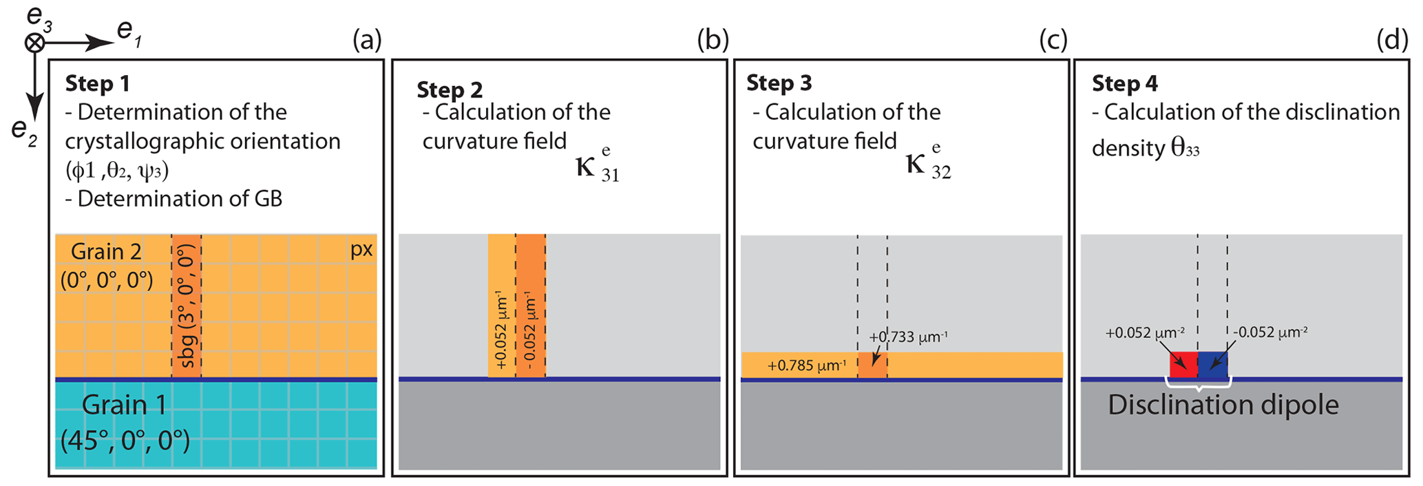
Figure 1 Sketch illustrating an example of the calculation of the wedge disclination θ₃₃ along a grain boundary. (a) Two grains with orientations given by Euler angles at 45^∘, 0^∘, 0^∘ (grain 1) and at 0^∘, 0^∘, 0^∘ (grain 2), which define a pure tilt grain boundary (GB) of misorientation > 5^∘. A sub-grain is inserted within grain 2 with a disorientation of 3^∘ around axis e₃. (b) The field of the $K_{\mathrm{31}}^{\mathrm{e}}$ component of the curvature tensor is derived by one-sided differentiation of field of the ${\mathit{\omega }}_{\mathrm{3}}^{\mathrm{e}}$ component of the elastic rotation vector. (c) The field of the $K_{\mathrm{32}}^{\mathrm{e}}$ component of the curvature tensor is derived by forward differentiation of ${\mathit{\omega }}_{\mathrm{3}}^{\mathrm{e}}$. (d) The density of wedge disclinations θ₃₃ is derived from forward differentiation of the field of the $K_{\mathrm{31}}^{\mathrm{e}}$ and $K_{\mathrm{32}}^{\mathrm{e}}$ components of the curvature tensor. Redrawn after Fressengeas and Beausir (2018; their Fig. 2).

An application of this calculation is shown in Fig. 2 for the small section of the starting-material EBSD map (sample CMT-16-7), where disorientation gradient pixel per pixel can be seen along grain boundaries. As this scale of investigation is impractical to compare large EBSD maps, smoothing is applied to ease the display and to reach a certain level of visual comfort (i.e., compatible with publication format). Smoothing too much strongly affects the displayed width of disclination monopoles and dipoles, as shown by Fig. 2b–e, to the point where it gives the false impression that the disclination is “crosscutting” the grain boundary. Nonetheless, only non-smoothed data are used for the density calculations (Fig. 2a). A smoothing factor of 2 was found to be appropriate to yield the best display of the EBSD maps investigated here.

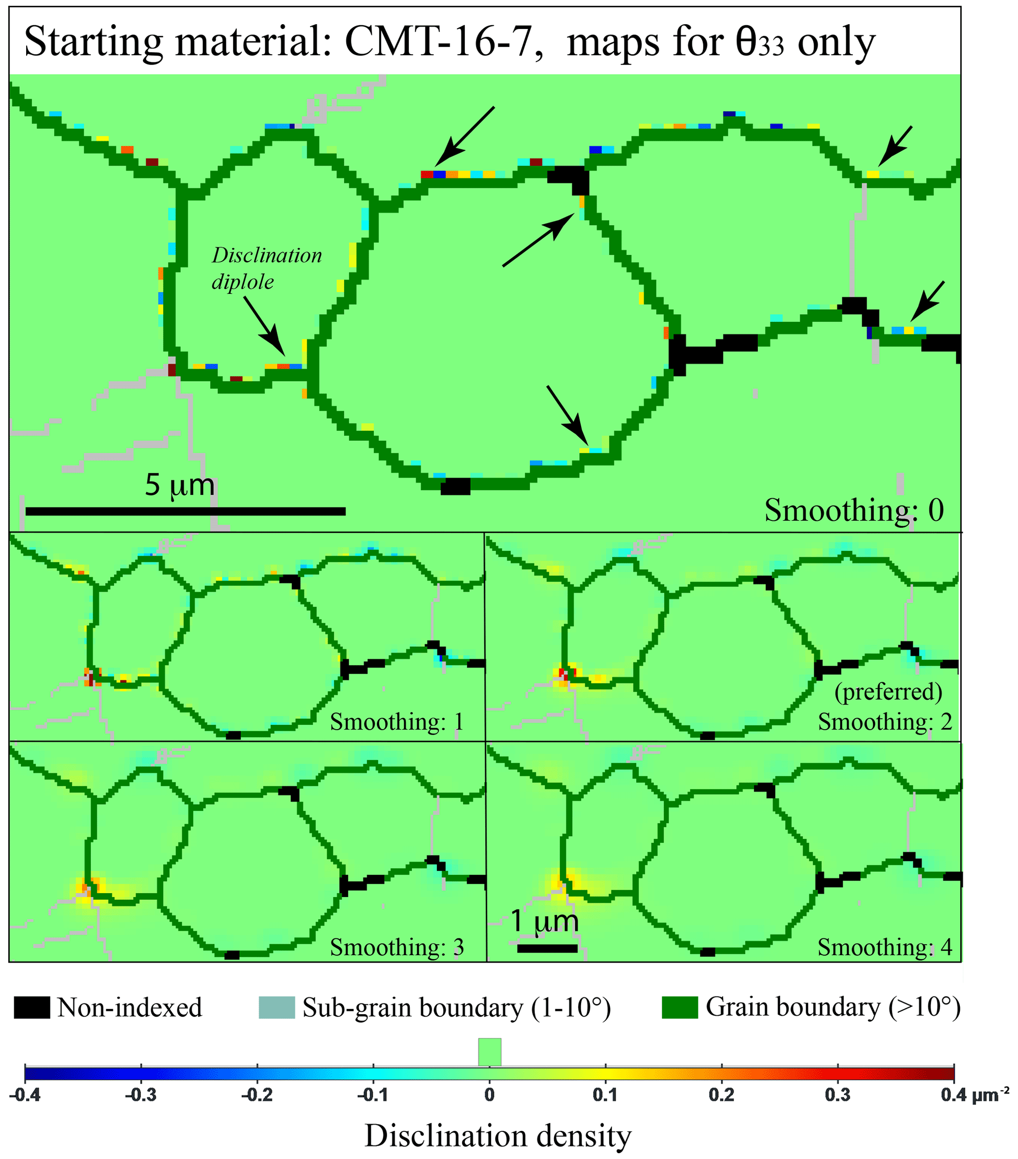
Figure 2 Comparison of wedge disclination densities θ₃₃ with different smoothing factors of 0, 1, 2, 3, and 4, for a selected area (top left corner) of the starting-material map (sample CMT-16-7). A user-defined scale was used here; the step size was 0.1 µm, and the range of disorientation for disclination detection was 0–10^∘.

While the chosen smoothing treatment does not impact disclination densities, the chosen range of disorientation, e.g., 0–1, 0–5, or 0–10^∘, does impact the output disclination densities. As expected, a larger disorientation range (0–10^∘) yields higher disclination densities than a restrain range (e.g., 0–5^∘) as it acts as a cutoff. Furthermore, a fine range of disorientation (0–1^∘) is a necessity to visualize disclinations along sub-grain boundaries, and a large range of disorientation (0–25^∘) only highlights major disclinations at triple junctions (major sub-grain boundaries). The effect of disorientation range for disclination identification (and thus quantification) is illustrated by Fig. 3 on a relatively large olivine grain (6–8 µm), with crosscutting sub-grain boundaries in the selected area of starting material (CMT-16-7, left edge of the original map). A range of 0–10^∘ of disorientation is found appropriate for our samples to best identify the disclination population along the grain boundaries. This choice is also consistent with the 10^∘ used to define grain boundaries.

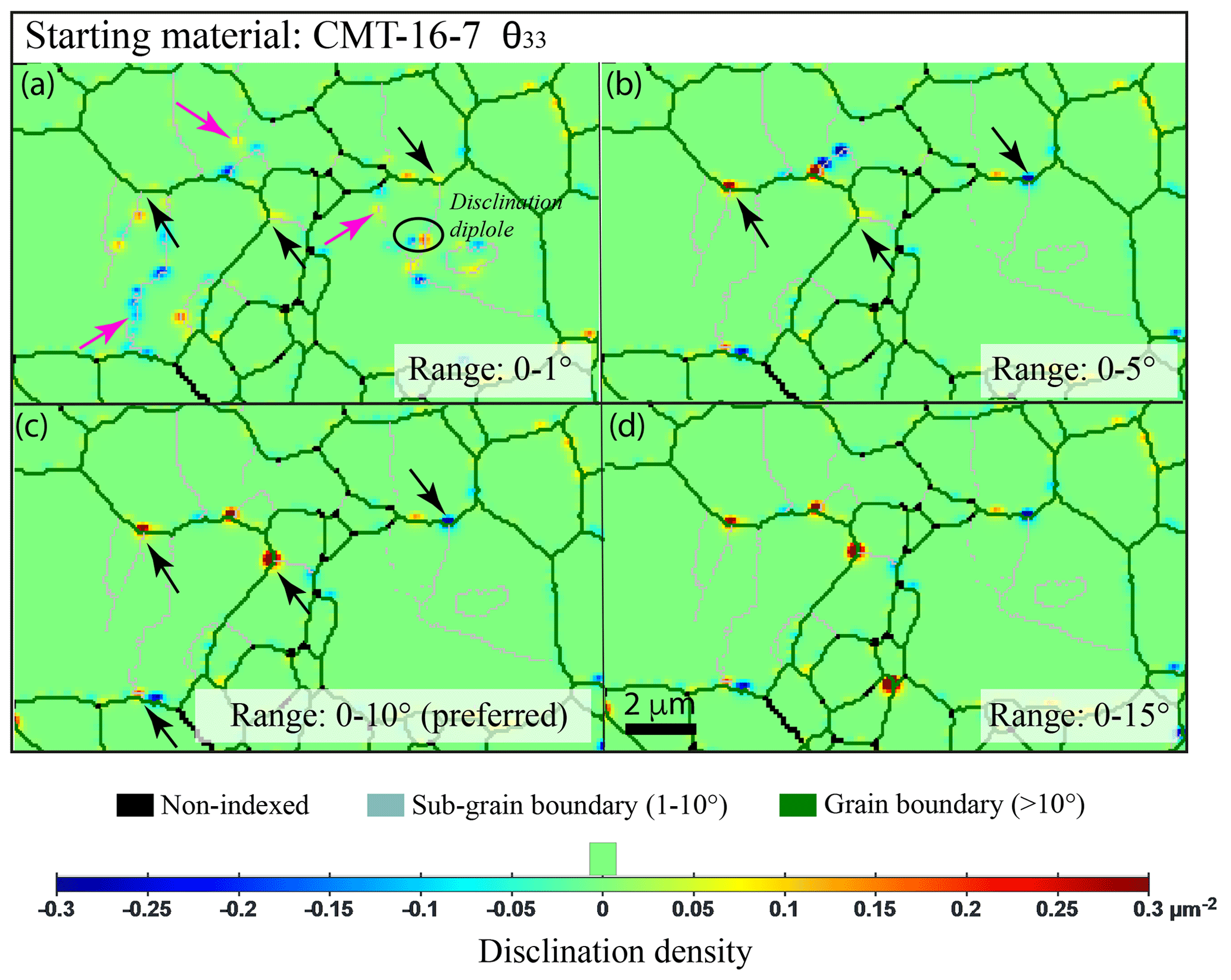
Figure 3 Comparison of wedge disclination densities θ₃₃ with a different range of disorientation for disclination detection for the selected area (left edge) of the starting-material map (sample CMT-16-7). A user-defined scale was used here; the step size was 0.1 µm, and the smoothing factor was 2. Black arrows indicate disclination at triple junctions or grain boundary–sub-grain boundary junctions, and the pink arrows indicate disclination at the intragranular tip of sub-grain boundaries.

Once disclinations are detected, the densities can be calculated, but from a two-dimensional map, only θ₁₃, θ₂₃, and θ₃₃ can be obtained. Nevertheless, we emphasis that, to date, ATEX is the only piece of software able to provide such quantification. The average disclination density is noted ρ_θ and corresponds to the entrywise norm of the respective matrix. As mentioned above, the maps are only two-dimensional; thus we stress that the entrywise norm is only a partial representation of the “true” disclination density (three non-null components out of nine components), not rotated in the crystal framework. Nevertheless, the entrywise norms obtained in the sample framework or crystallographic framework yield identical values. As the crystallographic control on Frank's vector (ω) and its magnitude are still unknown for olivine, in the simplified system considered here, we take

$$\begin{array}{}\text{(6)}& {\displaystyle }{\mathit{\theta }}_{ij}=e_{jkl}{\mathit{\kappa }}_{il,k}^{\mathrm{e}},\text{(7)}& {\displaystyle }{\mathit{\rho }}_{\mathit{\theta }}=\sqrt{\left({\mathit{\theta }}_{\mathrm{13}}^{\mathrm{2}}+{\mathit{\theta }}_{\mathrm{23}}^{\mathrm{2}}+{\mathit{\theta }}_{\mathrm{33}}^{\mathrm{2}}\right)}.\end{array}$$

We recommend adjusting the scale individually (e.g., user-defined mode) for each map first before choosing a common user-defined scale. A sample area with very low disclination densities blends in with the colored background. Adjustments and trade-offs are a necessity to best visualize the treated maps. For our set of maps, the best setup is a range of disorientation of 0–10^∘ (as defined for grain boundary) and a user-defined scale of −0.5 to +0.5 rad µm⁻² for disclination norms. As for the smoothing factor, the choice of an auto-scale or user-defined scale (linear or log) does not affect the calculated GND or disclination densities; only the display is affected.

For EBSD maps which were acquired at step sizes < 0.1 µm (Table 2), ${\mathit{\rho }}_{\mathit{\alpha }}^{\mathrm{c}}$ and ρ_θ were calculated for the original step size. Furthermore, the same maps were sampled again for analysis to reach a step size of 0.1 µm and to permit accurate comparison with the other EBSD maps. Furthermore, the map sample CMT-16-13-SII was sampled again for a step size of 0.2 µm to further assess the importance of step size on both ${\mathit{\rho }}_{\mathit{\alpha }}^{\mathrm{c}}$ and ρ_θ quantification. At last, ATEX generated statistics of GND and disclination (DCL) (1) per pixel and (2) per grain (one point per grain, oppg). Resulting densities for a given map are thus not identical if acquisition step size was different. The average density per map based on average density per grain can be calculated, but we also provide the median density per grain for each map. Comparison between average and median densities show that median densities are more accurate representations of distribution when compared to average densities (see Table 2).

In recent years, disclinations have gained visibility in metal and minerals and disconnections too (Hirth and Pond, 1996; Beausir and Fressengeas, 2013; Cordier et al., 2014; Sun et al., 2016; Fressengeas and Beausir, 2018; Sun et al., 2018, 2019; Hirth et al., 2019, 2020). We recall here that the type of EBSD (orientation) maps used in this study allow for estimating standard (Volterra) disclination defects, involving a discontinuity of elastic rotations. Very recently, Hirth et al. (2020) introduced the concept of coherency disclinations, which can occur at terminating coherent interfaces (or terraces) or slant facets as large step disconnections. Investigating the possible occurrence and the associated elastic fields of such defects in olivine could be possible by combining HR-EBSD (high-angular-resolution electron backscatter diffraction; giving then access to elastic strains in the maps) and a recent continuum mechanics framework of generalized disclinations (Acharya and Fressengeas, 2012; Berbenni et al., 2014). Furthermore, atomic-scale modeling would be required to investigate the precise topology and dynamics of such defects. However, we recall that to date, disconnections were never observed as constituent defects of olivine grain boundaries, using transmission electron microscopy, for example, and that a framework explaining their potential mobility still does not exist (e.g., Cahn et al., 2006). On the other side, Volterra disclination identification by TEM was recently proposed by Idrissi et al. (2022), and a mobility framework was already established (e.g., Acharya and Fressengeas, 2015; Taupin et al., 2013, 2014; Combe et al., 2016).

2.2.4 Numerical estimation of internal elastic energy induced by GND and disclination densities

To further probe the relative roles of dislocations and disclinations in the accommodation of plastic deformation, we will use the GND and disclination densities, as measured by EBSD, as inputs in two-dimensional field dislocation and disclination mechanics (FDDM) simulations previously developed by Fressengeas et al. (2011). The field equations (incompatibility equations, balance-of-stress equation) are numerically solved with spectral solvers based on fast Fourier transform (FFT). The methodological details can be found in previous studies (Berbenni et al., 2014; Djaka et al., 2017; Berbenni and Taupin, 2018). In the simulations presented later, the FFT grid size is the same as the EBSD map step size. For a given region of interest selected on an EBSD map, inputs in the simulations will be the orientation of each grain (Euler angles) and the GND and disclination densities. Elastic coefficients in the olivine crystal frame (Pbnm) are C₁₁₁₁=320.2, C₂₂₂₂=195.9, C₃₃₃₃=233.8, C₂₃₂₃=63.5, C₁₃₁₃=76.9, C₁₂₁₂=78.1, C₁₁₂₂=67.9, C₁₁₃₃=70.5, and C₂₂₃₃=78.5 GPa (as in Cordier et al., 2014). For a selected EBSD map, four different simulations are calculated, namely (i) a simulation with no defect but with applied axial loading (like the experimental one) to see the effect of crystalline elastic anisotropy on the distribution of energy, (ii) a simulation with only GND densities and no loading, (iii) a simulation with only disclination densities and no loading, and (iv) a simulation with both GND and disclination densities and no loading. In the simulations with no loading, all stress components are imposed to be null macroscopically (only one component is assigned to a very small value to ensure convergence of the spectral algorithm). Periodic boundary conditions are present in all directions due to the use of Fourier transforms. As such, care should be taken in the analysis of the simulated mechanical fields distribution, and one should rather consider fields in the center of the simulation domains and not those near the map boundaries. Nevertheless, the predicted mechanical fields allow here for investigating qualitatively the concurrent role of GND and disclination densities in accommodating plastic deformation of olivine. From initial dislocation/disclination inputs, the FDDM simulations give here as outputs the elastic strains and rotations, the internal stresses (Cauchy stress tensor), the elastic curvatures, and the local elastic-energy density in the microstructure modeled. Note that FDDM can further be used to simulate the transport of defect densities during plastic straining. In this preliminary FDDM analysis, we will compare the distributions of the internal elastic energy for the four cases mentioned above to evidence the interplay between disclinations and dislocations.

3 Results

3.1 Microstructures

We compile below the statistical results from the new EBSD investigation; it complements previous studies (Demouchy et al., 2012; Thieme et al., 2018). Forward-scattered electron images representative of the starting material (CMT-16-7) and samples from uniaxial compression at 1000 ^∘C (CMT-17-2) from uniaxial compression at 1200 ^∘C (CMT-16-9) and from torsion experiment at 1200 ^∘C (PI0546) are presented in Fig. 4. All samples are composed of olivine at 99.8 %; enstatite and Cr-spinel only represent < 0.2 % in the studied area. Grains are sub-equant; the average olivine grain size is homogeneous trough the data set and ranges from 1.3 to 2.7 µm. The mean aspect ratio is 1.4–1.5, and the maximum aspect ratios are up to ∼ 3.0. Grain boundaries are curved and/or serrated, and only a hint of grain boundary migration is observed (i.e., grain growth at the expense of the most highly misoriented neighboring grains), which is also observed in the starting material (CMT-16-7, Fig. 4a). A few grains show residual internal micro-cracks oriented at 60^∘ to each other, which are also present in the starting material and which are attributed to thermal cracking during quench. Actually, there is no significant displacement or sliding along these cracks. A low fraction of porosity (2 %–5 %) is apparent in Fig. 4, which is mostly inherited from the notorious imperfect hot pressing at 300 MPa, even for a very fine grain size of olivine (e.g., Beeman and Kohlstedt, 1993; Zimmerman and Kohlstedt, 2004; Demouchy et al., 2014; Hansen et al., 2012; Warren and Hirth, 2006). The initial low porosity is also overestimated due to grains plucking during the polishing stages.

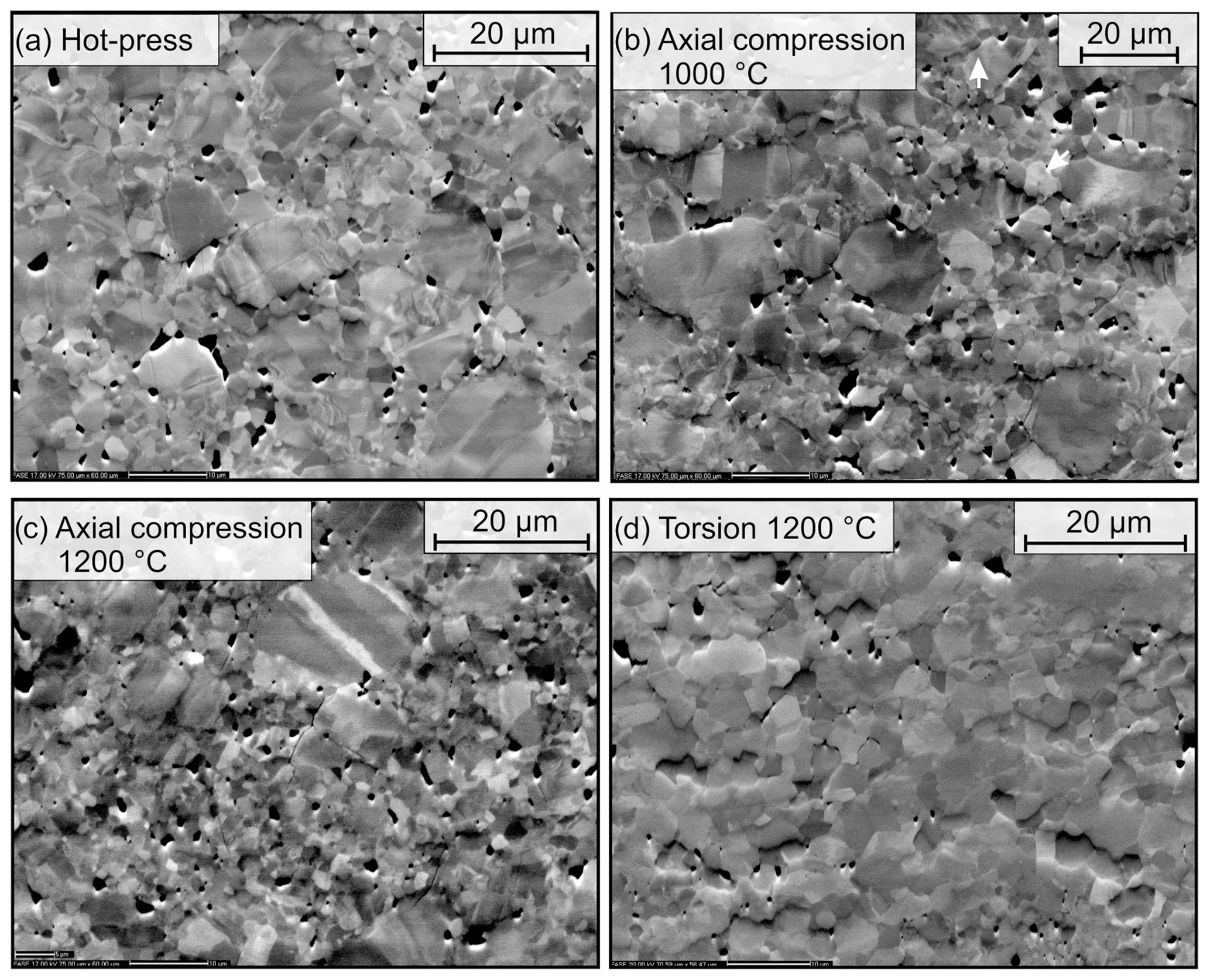
Figure 4 Forward-scattered electron images from scanning electron microscopy (SEM). (a) Typical image from starting material, undeformed but sintered aggregate by hot pressing at high temperature and pressure (sample CMT-16-7). (b) After axial compression at 1000 ^∘C and for 7.3 % of finite strain (CMT-17-2). (c) After axial compression at 1200 ^∘C and for 8.6 % of finite strain (CMT-16-9). (d) After torsion at 1200 ^∘C and for 2.05 % of equivalent strain (PI0546). Dark areas are pluck-outs from polishing and residual pores from the hot-press step (see main text for details).

The conditions of the deformation experiments and mechanical results are recalled in Table 1, while the new acquisition indexation rate, step size, number of identified grains, average grain size, ${\mathit{\rho }}_{\mathit{\alpha }}^{\mathrm{c}}$, and ρ_θ for each of the 19 EBSD maps are given in Table 2. The indexation rates for our EBSD maps are at least 90.9 % and up to 97.9 %.

3.2 GND and disclination identification and their densities

An example of GND identification and distribution in the crystallographic frame is provided in Fig. 5 for sample PI0456-XIV (full map displayed). Dislocation types in the crystallographic framework (${\mathit{\alpha }}_{ij}^{\mathrm{c}}$) and corresponding olivine slip systems ([uvw](hkl)) are both indicated in the figure. The correspondence is recalled in Table 3 but only for the main slip systems in olivine (see further details in Mussi et al., 2014). GND distribution is heterogeneous, and as expected, the highest densities are observed along well-developed sub-grain boundaries but with a mixed character, made of both [100] and [001] dislocations. From the full data set, the average one-point-per-grain GND density ranges between 2.25 × 10¹¹ and 5.28 × 10¹¹ m⁻² (Table 2 for 0.1 µm step size). One of the minimal dislocation densities is found for the starting material, which is 2.6 × 10¹¹ m⁻². The same distribution is found when comparing median values (Table 2). The highest density is observed in a sample deformed at low temperature and high stress (1000 ^∘C, sample CMT-17-2). Note that the minimum dislocation density from all maps (0.1 µm step size) is 2.0 × 10¹⁰ m⁻² on average. Furthermore, average ${\mathit{\alpha }}_{\mathrm{1}j}^{\mathrm{c}}$ densities are rather similar to ${\mathit{\alpha }}_{\mathrm{3}j}^{\mathrm{c}}$ (Table S1). The GND densities do not clearly vary between samples deformed in uniaxial compression or in torsion with comparable stresses, finite strains, and the number of grains (Table 2). The most deformed sample at 1000 ^∘C (CMT-17-2) has a higher GND density than the most deformed sample at 1200 ^∘C (CMT-16-9) for a similar strain rate (∼ 1 × 10⁻⁵ s⁻¹), and both have higher GND densities than the starting material (Table 2).

Table 3 Dislocation type, corresponding slip systems, and GND in the crystallographic frame (${\mathit{\alpha }}_{ij}^{\mathrm{c}}$).

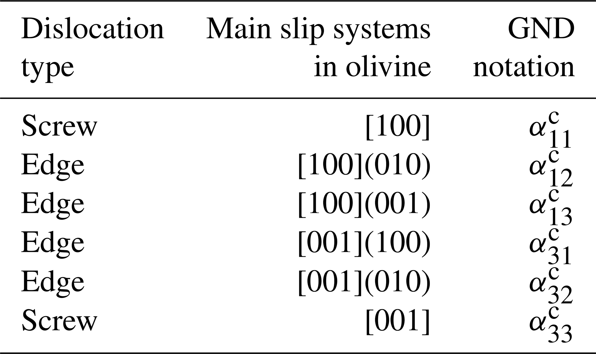
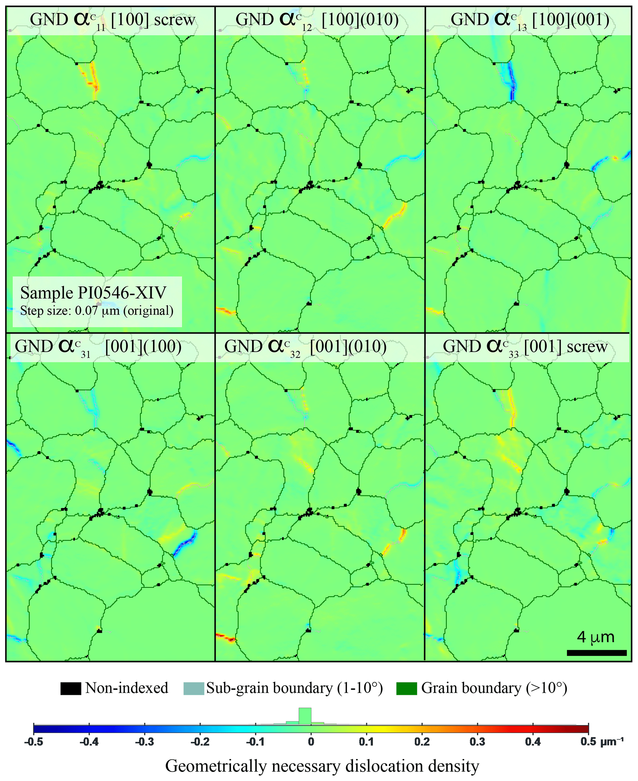
Figure 5 Representative distribution of the different GND densities reported in the crystallographic frame (noted α^c) in the sample deformed in torsion (PI0546-XIV). The density scale is automatically set up for this set of maps; the step size was 0.07 µm (original acquisition step size), and the smoothing factor was 2.

From the same sample (PI0456-XIV), the typical disclination type and spatial distribution are shown in Fig. 6. Disclination monopoles and dipoles are located along grain boundaries and with a distinctive occurrence at a junction between a sub-grain boundary and a grain boundary (black arrows in Figs. 3 and 6). Furthermore, disclinations are also found at the intracrystalline tip of sub-grain boundaries (pink arrows) as shown in both the starting material (Fig. 3) and in experimentally deformed samples. We show another example in Fig. 7 but for a larger range of disorientation for the disclination detection. For a distinctive range of disorientation (e.g., 0.1 or 0–5^∘), disclinations can occur as strings of monopoles along sub-grain boundaries (Fig. 3b). Overall, throughout the data set, the one-point-per-grain disclination density ranges from 7.3 × 10⁻³ to 6.5 × 10⁻² rad µm⁻² (Table 2). As for GNDs, there is no linear variation (increase or decrease) between samples deformed in uniaxial compression or in torsion with comparable stresses. However, the most deformed sample at 1000 ^∘C (CMT-17-2) has a higher disclination density than the most deformed sample at 1200 ^∘C (CMT-16-9) for similar strain rate (∼ 1 × 10⁻⁵ s⁻¹) but only by a factor of 1.4.

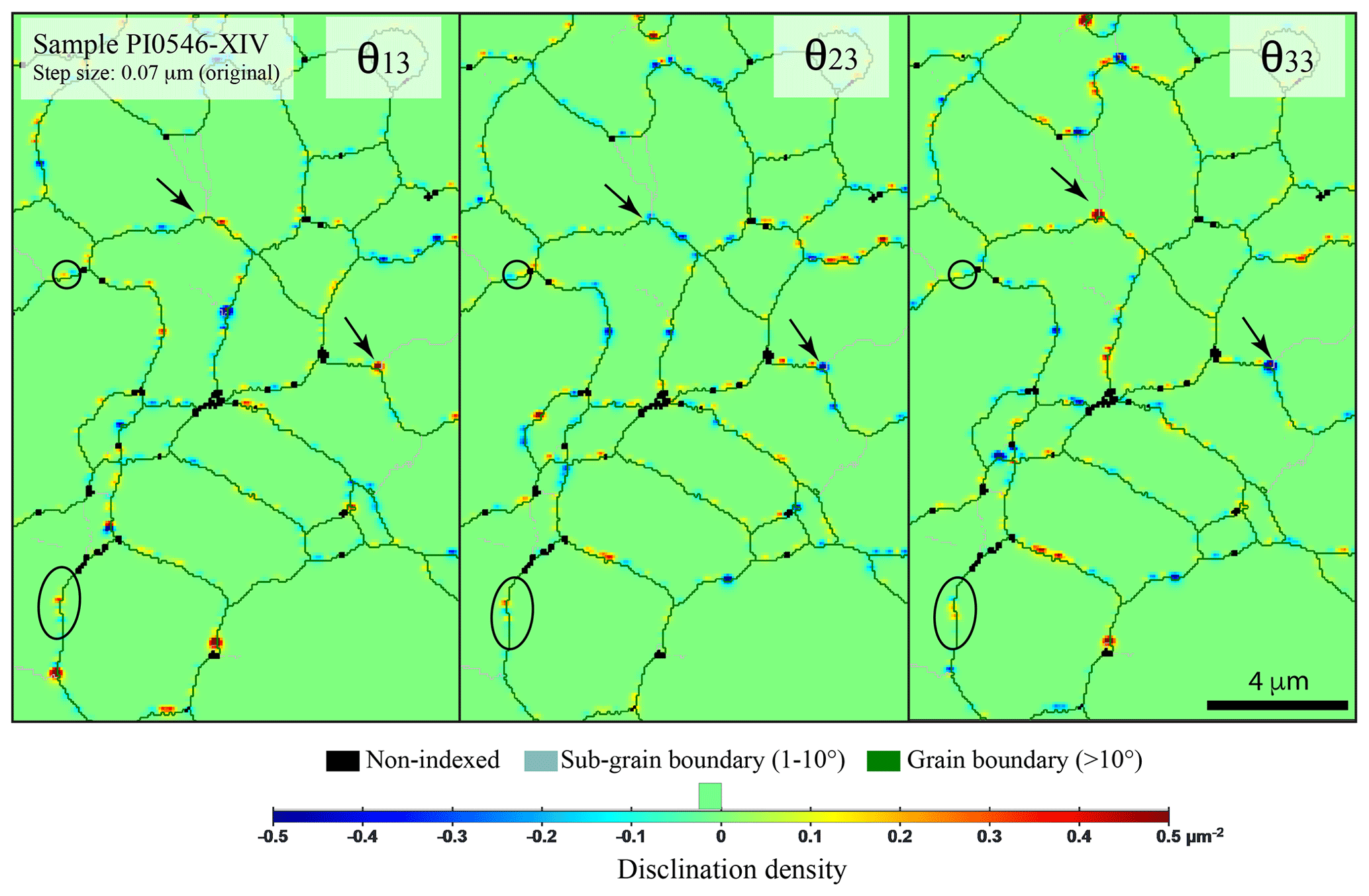
Figure 6 Representative distributions of the different disclinations (θ₁₃, θ₂₃, and θ₃₃) reported in a sample deformed in torsion (PI0546-XIV). Circles indicate well-defined dipoles after smoothing. Arrows indicate dipoles at the junction between a sub-grain boundary and a grain boundary. The density scale is user-defined for this set of maps; the step size was 0.07 µm, and the smoothing factor was 2.

3.3 Impact of step size

For both GNDs and disclinations, special attention was given to the impact of step size for accurate comparison while keeping the step size small enough (≤ 0.1 µm) for accurate detection of variation in the disorientation gradient along grain boundaries. The effect of the step size on the resulting GND and disclination densities is shown in Fig. 8. As expected, both GND and disclination densities are strongly dependent on the spatial resolution of the EBSD map. Here GND and disclination distributions are shown for sampling at a relatively large step size of 0.1 and 0.2 µm. The maps are displayed here with a fixed user-defined scale (i.e., −0.5 to +0.5 µm⁻¹ for GND and −0.5 to +0.5 rad µm⁻² for disclination). We selected to show ${\mathit{\alpha }}_{\mathrm{31}}^{\mathrm{c}}$ corresponding to edge [001](100) dislocations as an example here, but a similar decrease in dislocation density is observed for ${\mathit{\alpha }}_{\mathrm{1}j}^{\mathrm{c}}$ (cf. Table S1). Disclination θ₃₃ is chosen again for the illustration of the acquisition step size impact. Doubling the step size twice (from 0.05 to 0.2 µm) results in a decrease by a factor of 4 for ${\mathit{\rho }}_{\mathit{\alpha }}^{\mathrm{c}}$ and a drastic decrease by a factor of 16 for ρ_θ as reported in Table 2 and displayed in Fig. 9. The decrease is not linear, clearly showing the necessity of a very fine step size (≤ 0.1 µm) compared to the commonly used 0.25–1.0 µm step size (even with high-angular-resolution EBSD, e.g., Wallis et al., 2016, 2017). The evolution of the densities also shows that even for these small step sizes, densities do not reach plateau values, an observation also made recently in natural olivines by Ma et al. (2022). Our results also illustrate the difficult trade-off between spatial resolution (≤ 0.1 µm), angular resolution (≤ 0.5^∘), and the final size of the EBSD map to properly characterize a sample with sound statistical meaning.

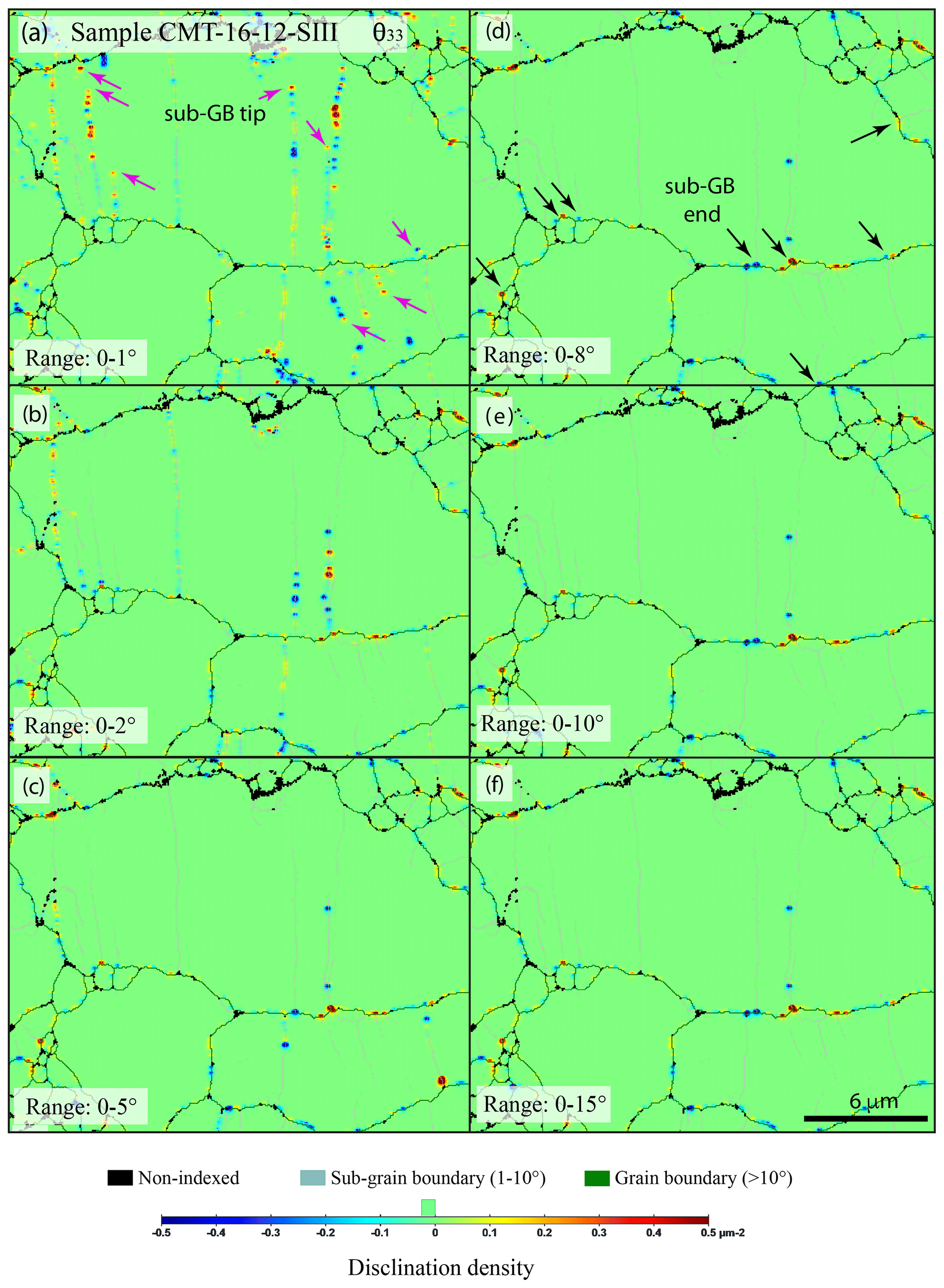
Figure 7 Comparison of wedge disclination densities θ₃₃ with a different range of disorientation for the full EBSD map from a sample deformed in axial compression (sample CMT-16-12, 1200 ^∘C, low strain ∼ 1 %) centered on a large olivine grain. A user-defined scale was used here; the step size was 0.06 µm, and the smoothing factor was 2. Black arrows indicate disclination at triple junctions or grain boundary–sub-grain boundary junctions, and the pink arrows indicate disclination at the intragranular tip of sub-grain boundaries.

Figure 8 Representative distribution of GND (${\mathit{\alpha }}_{\mathrm{31}}^{\mathrm{c}}$) and disclinations (θ₃₃) for the following values of step size in a sample deformed in axial compression (CMT-16-13-SII, 1200 ^∘C, low strain ∼ 3.7 %) centered on a large olivine grain: 0.05 µm (original step size), 0.1 µm (new sampling), and 0.2 µm (new sampling). The density scale is user-defined and the same for this set of maps; for both GND and disclinations the smoothing factor was 2.

3.4 GND distribution and grain size

The average grain size is small (2 µm) and relatively homogeneous across the data set, with a lognormal distribution and not a constant value. We tentatively explore the relationship between the GND densities and the grain size for this limited grain size range (0.2–20 µm) and low finite strains (Table 1). The GND densities in olivine as a function of grain size is displayed in Fig. 10a for four maps (all for a step size of 0.1 µm) from the starting material (CTM16-7), the sample deformed in axial compression at low temperature (1000 ^∘C) and the highest stress (CMT-17-2), the sample deformed in axial compression at high temperature (1200 ^∘C) and the highest strain (CMT-16-9), and for one sample deformed in torsion for the largest maps (PI0546-III, over 770 grains). The corresponding data set is given in Table S1. The data are scattered and do not show a distinct positive correlation between one-point-per-grain GND densities and grain size. However, the average GND density in the starting material is lower (2.6 × 10¹¹ m⁻²) than in the deformed sample in compression (sample CMT-17-2-SII, 5.3 × 10¹¹ m⁻²; sample CMT-16-9-SII, 3.6 × 10¹¹ m⁻²) or in the deformed sample in torsion (sample PI0546-III, 3.9 × 10¹¹ m⁻²). The difference in GND density is less than 1 order of magnitude, though it approaches a substantial factor of 2. For the four samples considered in Fig. 10a, we further show the distributions of the average GND density per grain in Fig. 10b (for a fixed number of bins at 50, whatever the number of grains), which demonstrates a distribution close to a lognormal one and which indicates that the use of a median value instead of a crude average from the average per grain would be preferable (see Tables 2 and S1 for a comparison of numerical values).

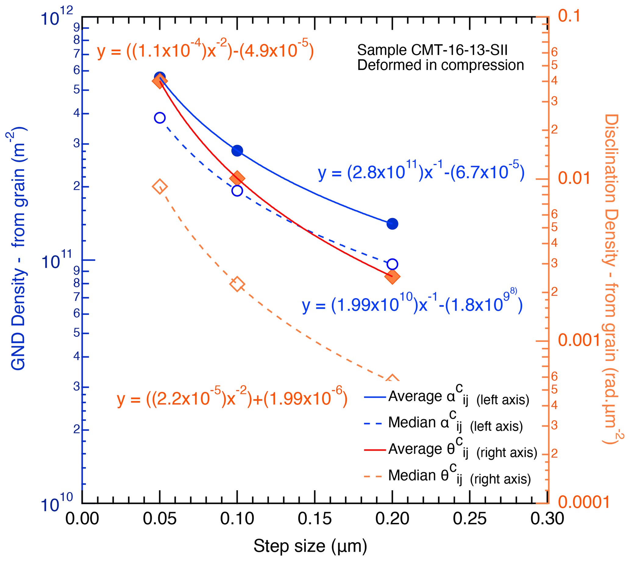
Figure 9 Resulting variation in average and median densities (from an one-point-per-grain data set) of GND and disclination densities as a function of the EBSD acquisition step size from 0.05 µm (original step size) to 0.1 µm (new sampling) and 0.2 µm (as displayed in Fig. 8).

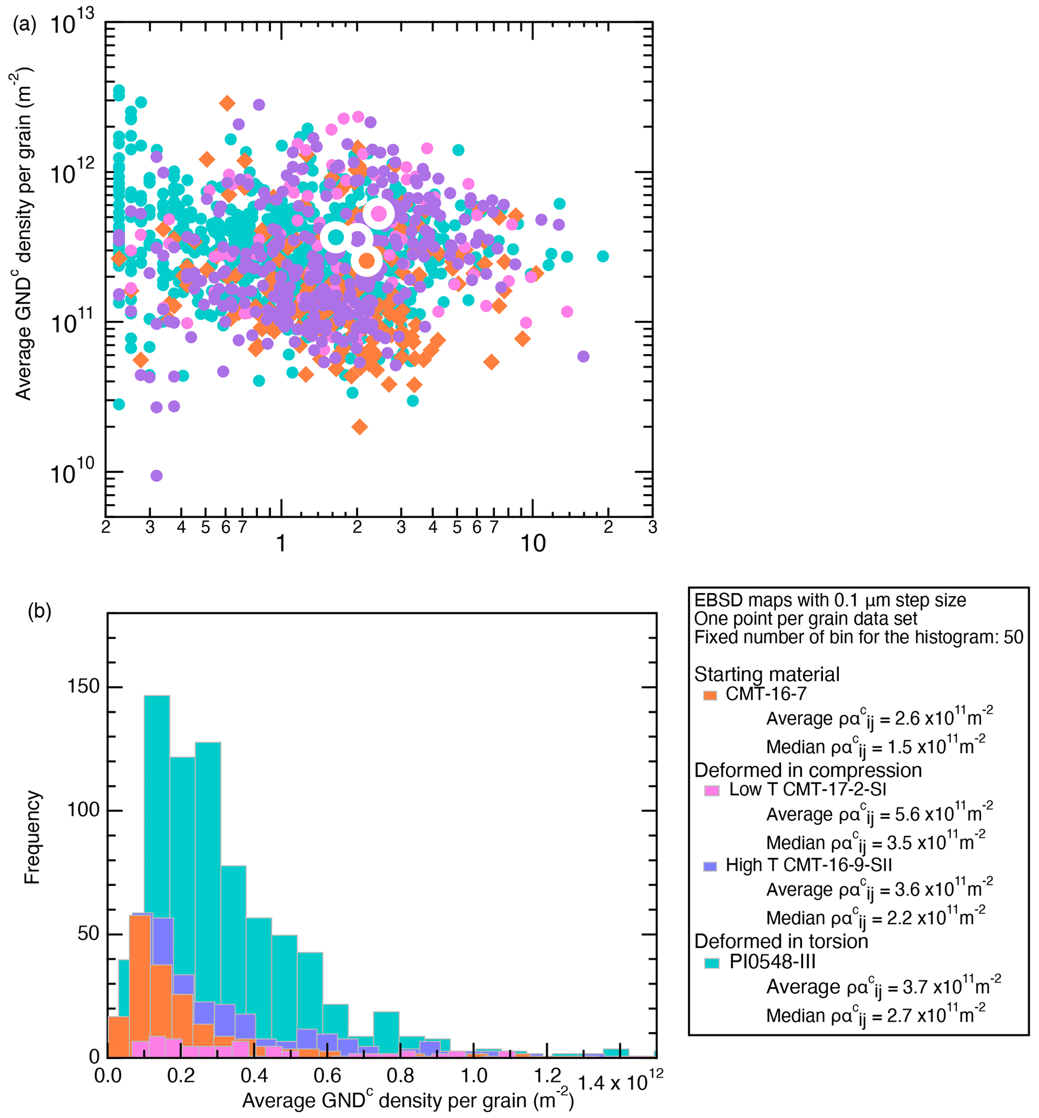
Figure 10 (a) Representative distribution of GND density (one point per grain) as a function of the grain size in the starting material (CMT-16-7), in two samples deformed in axial compression (at low temperature for CMT-17-2 and at high temperature for CMT-16-9-SII) and in a sample deformed in torsion (PI0546-III). The step size was 0.1 µm (original acquisition step size). Also shown is the average GND density for each sample as a large symbol; (b) same samples as in (a) with a histogram of GND density (one point per grain) showing a distribution close to lognormal, with the median values then representing the distribution more accurately than the average densities.

While the extracted densities permit exploring limited statistical parameters, one of the complementary approaches is also to compare dislocation distributions in maps visually. Is one able to see in the maps the dislocation density difference observed in average and median densities between the low- and high-temperature deformation in axial compression? We illustrate the answer with Fig. 11, which shows two ways to display the GND norm. Figure 11a and b are identical, and Fig. 11c and d are also identical. Only the color scale is different; in blue, we used the MATLAB classic linear color scale “jet” (“rainbow” in ATEX, starting with blue, with a smoothing factor of 2), which is also used typically for KAM (kernel average misorientation) maps, and in green we used a log scale (“linear green” in ATEX, with a smoothing factor of 1). A higher density in GND and more grains with numerous GNDs for the sample deformed at lower temperature are visible in Fig. 11, confirming the veracity of value extracted from the map (Table 2). Furthermore, one can easily differentiate two types of GNDs with the green color scale, while they remain very subtle using the classic jet/rainbow color scale. A major one (white arrows) defines, as expected, the well-defined sub-grain boundaries, but also a second type, widespread (e.g., dashed pink circles in Fig. 11c and d), not homogeneous but practically ubiquitous, defines an almost polygonal structure like the one observed during dynamic recrystallization. The high-temperature sample still displays GND-poor small grains, while in the sample deformed at low temperature, even small grains have high GND densities. Even if GNDs are a mere proxy for average mobile dislocation, in this specific case and qualitatively, the method remains discriminant and in agreement with Orowan's law. Although, the reliability of the numerical densities remains to be examined.

Figure 11 Representative distribution of the different entrywise norm of GND (major and minor type; see main text for details) with two different display strategy: (a) and (b) from a sample deformed in compression at high temperature and low stress (CMT-16-9) and (c) and (d) at low temperature and high stress (CMT-17-2). In (a) and (c), the classic jet color scale was used with a linear user-defined scale and a smoothing factor of 2; in (b) and (d) the linear-green color scale was used with a user-defined log scale and a smoothing factor of 1. The acquisition step size is 0.1 µm.

3.5 Disclination distribution and grain size

Since disclinations are distributed along grain boundaries or at sub-grains, correlation between the disclination densities and grain size is expected. To further assess the role of the grain boundary network (or grain size) in disclination abundance, disclination density is shown as a function of grain size or grain perimeter in Fig. 12a and demonstrates a broad negative correlation (following $y=x^{-\mathrm{1}}+b$). Furthermore, disclination densities are normalized to the perimeter (for a hypothetical spherical grain of diameter D with an area equal to the given grain) of each grain (thus in µm⁻³) as a function of the grain perimeter in Fig. 12b to better compare small and large grains. The correlation is enhanced for the four samples already selected for Fig. 10, but it is not identical. A linear least-squares fit through the log–log data for each sample yields a relationship similar for the four samples, including for the starting material. The latter displays a normalized disclination density of $f\left(x\right)=x^{-\mathrm{1.8}}$ × 10^−1.63, slightly lower than that for the three deformed samples for a similar perimeter range. Moreover, the global fit through the three deformed sample sets yields a distribution following $f\left(x\right)=x^{-\mathrm{2}}$ × 10^−1.3. This first approximation emphasizes the predominant occurrence of disclinations along boundaries in the smallest grains, even in the absence of noticeable dynamic recrystallization in this very fine-grained olivine aggregate (cf. Thieme et al., 2018). This result also shows a noticeable difference between the disclination density in the starting material (in CMT-16-7, median value of ${\mathit{\rho }}_{\mathit{\theta }}=\mathrm{4.08}\times {\mathrm{10}}^{-\mathrm{3}}$ rad µm⁻²) and in the deformed polycrystalline olivine (in PI0548, ${\mathit{\rho }}_{\mathit{\theta }}=\mathrm{7.12}\times {\mathrm{10}}^{-\mathrm{3}}$ rad µm⁻²). However, there is actually a negligible difference between the results from low- and high-temperature experiments in compression or torsion (median values for CMT-17-2 of ${\mathit{\rho }}_{\mathit{\theta }}=\mathrm{1.11}\times {\mathrm{10}}^{-\mathrm{2}}$ rad µm⁻², CMT-16-9 of ${\mathit{\rho }}_{\mathit{\theta }}=\mathrm{7.54}\times {\mathrm{10}}^{-\mathrm{3}}$ rad µm⁻², PI0548 of ρ_θ=7.12 rad µm⁻²). The inverse correlation (Fig. 12a) thus suggests that small grains would bare more disclination than relatively large grains in these fined-grained olivine samples, deformed or not deformed.

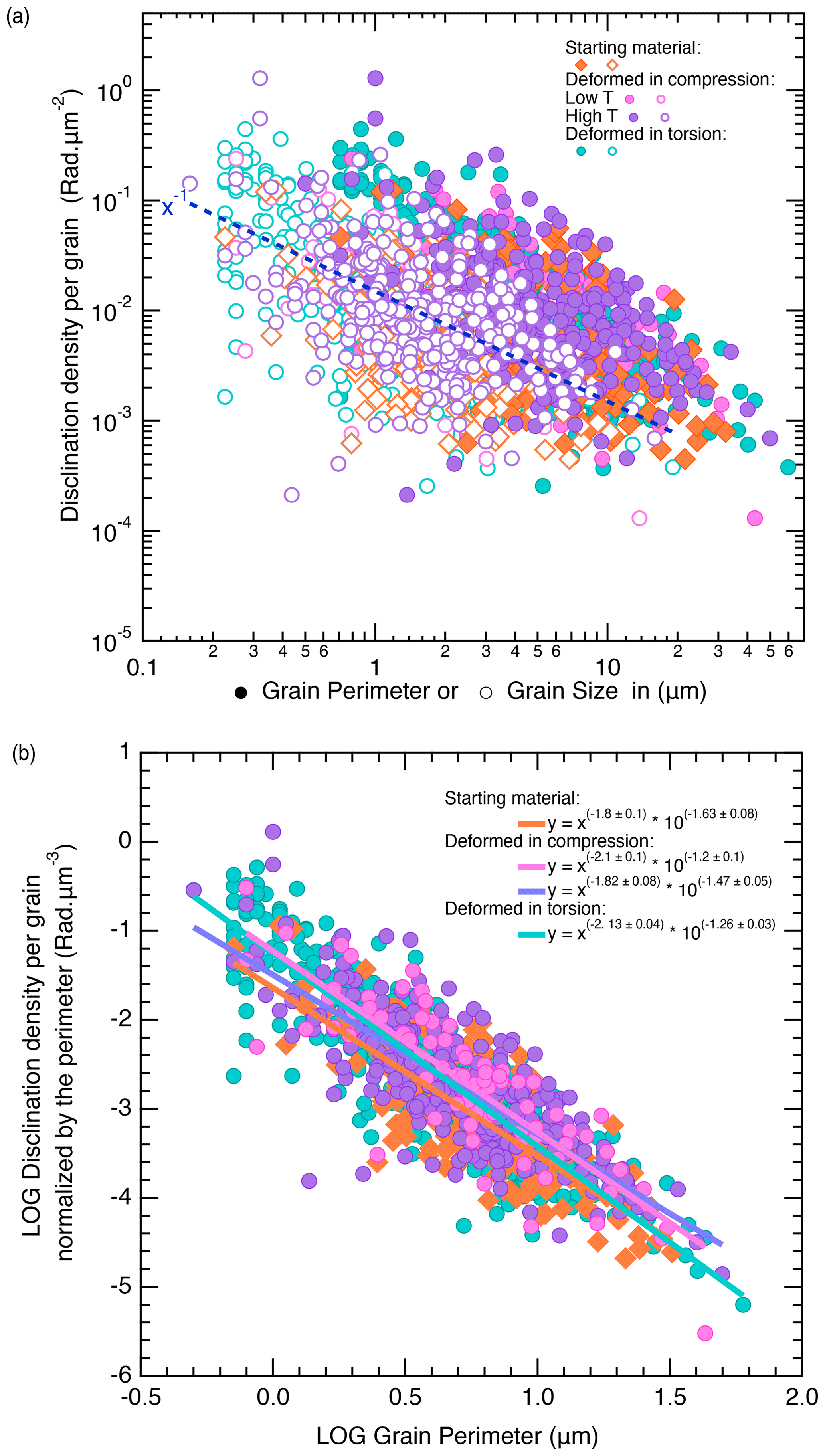
Figure 12 (a) Distribution of disclination densities (one point per grain) as a function of the grain size (hollow symbol) or grain perimeter (full symbol) in the starting material (CMT-16-7), in two samples deformed in axial compression (at low temperature for CMT-17-2 and at high temperature for CMT-16-9-SII) and in one sample deformed in torsion (PI0546-III). The step size is 0.1 µm (original acquisition step size). The dashed dark-blue line is a guide for the eye with a $y=x^{-\mathrm{1}}$ function. (b) Distribution of one-point-per-grain disclination densities normalized to the grain perimeter as a function of the grain perimeter in the starting material (CMT-16-7) in two samples deformed in axial compression (at low temperature for CMT-17-2 and at high temperature for CMT-16-9-SII) and in a sample deformed in torsion compression (PI0546-III). Also shown is the least-squares fit through each sample data set and the equation of the fit. See main text for details.

3.6 GND and disclination correlation

GNDs are usually seen as an indicator of the ductile deformation experienced by a polycrystalline material assuming that dislocation motion is the dominating parameter controlling creep and that a proportionality between GND and SSD is established (cf. Orowan's law, Hirth and Lothe, 1982; Wang et al., 2022). Since disclinations are also one-dimensional defects accommodating strain and we are now able to detect and quantify them, it is legitimate to question the respective role of these two types of defects (dislocations and disclinations) in the production of the strain and crystalline misorientation. Thus, we compare the GND and disclination densities in Fig. 13a and normalized to a grain size of sample PI-0546 in Fig. 13b. Since in this deformation experiment GND densities are not strongly dependent on grain size (Fig. 10a), the resulting broad and positive correlation is mostly driven by the grain size dependency of disclination densities (Fig. 12a, color coding in Fig. 13a) as observed in the starting material. Furthermore, in Fig. 13b the correlation is not matching a 1:1 line, indicating that the grain size effect is not similar for GND and disclination distributions. We remind the reader that the average grain size in all samples is rather small (2–3 µm); therefore such a distribution needs to be confirmed by studying a wider range of grain sizes and, if possible, one up to a geologically relevant olivine grain size (2–10 mm).

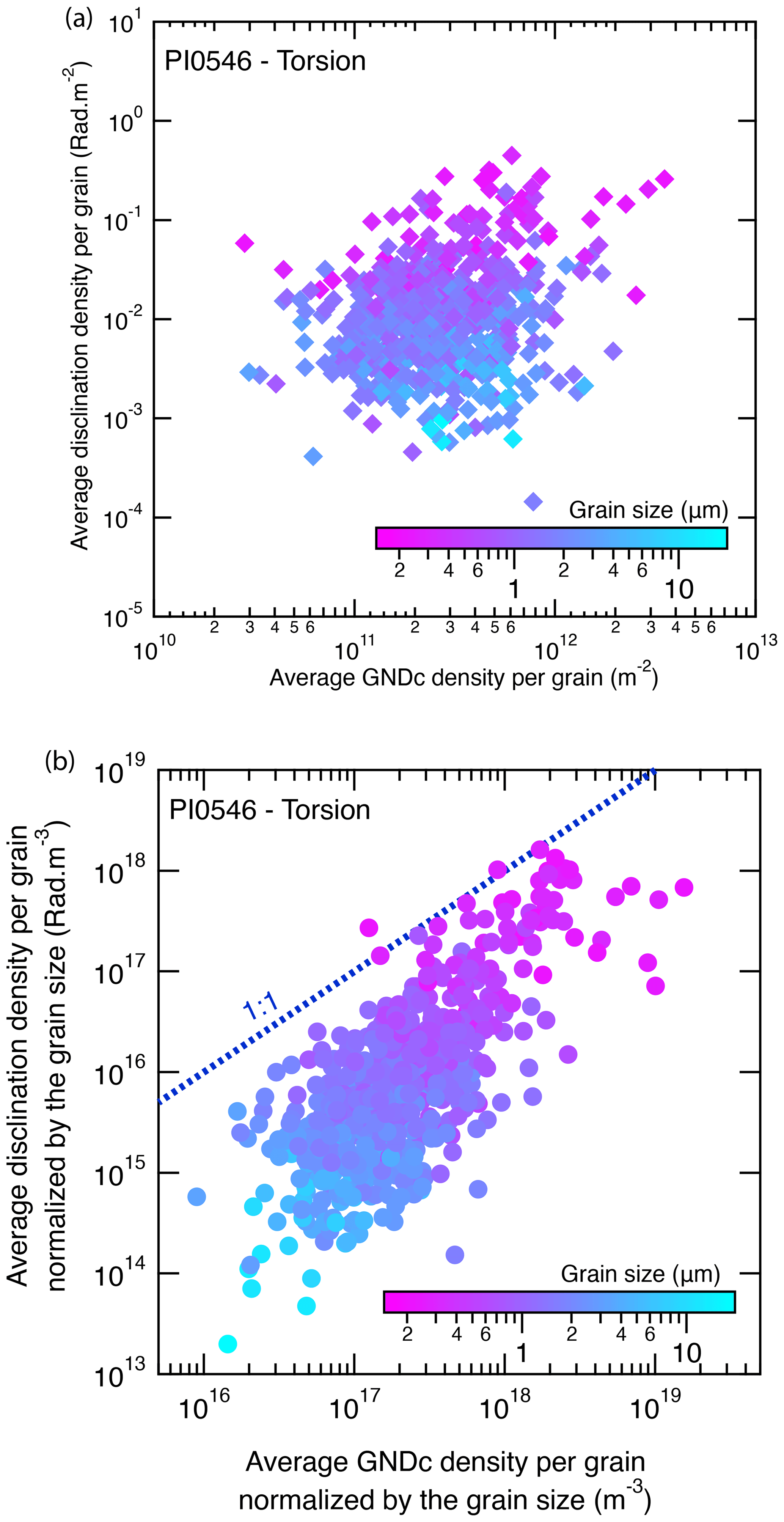
Figure 13 (a) Distribution of one-point-per-grain disclination densities as a function of the one-point-per-grain GNDc (${\mathit{\rho }}_{\mathit{\alpha }}^{\mathrm{c}}$) density for sample PI0546-III. (b) Distribution of one-point-per-grain disclination densities normalized to the grain size as a function of the one-point-per-grain GNDc density normalized to the grain size of sample PI0546-III. The data points are color-coded according to the associated grain size. The dashed dark-blue line is a guide for the eye with a 1:1 slope, showing that the correlation is not only due to grain size distribution. The step size is 0.1 µm (original acquisition step size).

4 Discussion

4.1 Occurrence of GNDs compared with previous studies

The calculation of the Nye tensor, followed by the rotation in the crystallographic frame of each grain permits the identification of the type of dislocations composing sub-grain boundaries, and the results show that, as expected, sub-grain boundaries are mostly built with dislocations of both [100] and [001] Burgers vectors, resulting in a boundary with a mixed character (neither perfect twist or tilt), as reported previously (e.g., Cordier et al., 2014; Wallis et al., 2017; Lopez-Sanchez et al., 2021). Despite the extremely rare presence to non-existence of [010] dislocation in olivine, here dislocations of the type $\mathit{\rho }{\mathit{\alpha }}_{\mathrm{2}j}^{\mathrm{c}}$ are present in the output results, with often a factor of 2 of difference as compared to $\mathit{\rho }{\mathit{\alpha }}_{\mathrm{1}j}^{\mathrm{c}}$ or $\mathit{\rho }{\mathit{\alpha }}_{\mathrm{3}j}^{\mathrm{c}}$ (Table S1). This result is at odds with decades of transmission electron microscopy (TEM) investigations but agrees with other EBSD studies mapping the Nye tensor (e.g., dislocations of α_2j in Fig. 2c in Cordier et al., 2014; dislocations of a₂₃ in Fig. 1 in Wallis et al., 2016). Here, we suggest that the occurrence of ${\mathit{\alpha }}_{\mathrm{2}j}^{\mathrm{c}}$ dislocations is interpreted as mere contributions from ${\mathit{\alpha }}_{\mathrm{11}}^{\mathrm{c}}$ and ${\mathit{\alpha }}_{\mathrm{33}}^{\mathrm{c}}$ screw dislocations components and not as a proof of the widespread existence of dislocations with such a long Burgers vector (cf. |b_l|=10.22 Å).

Furthermore, the distribution of the entrywise norm (Fig. 11; see also Fig. S1) still permits the inference of the presence of additional GNDs in between the array of major GNDs (cf. sub-grain boundaries), but these GNDs have a different spatial distribution than the well-oriented sub-grain boundaries within a given grain. A straightforward comparison of the distribution of minor GNDs between the polycrystalline sample deformed at 1000 ^∘C and high stress (1073 MPa, CMT-17-2) and the polycrystalline sample deformed at high temperature and lower stress (322 MPa, sample CMT-16-9) at a similar strain rate (∼ $\mathrm{1}\times {\mathrm{10}}^{-\mathrm{5}}$ s⁻¹) and level of strain (7.3 %–8.6 %) agrees with what is known from the hardening phenomenon during the creep mechanism at low temperature in olivine (800–1050 ^∘C). At these temperatures, recovery mechanisms (e.g., ionic self-diffusion, climb) are not efficient enough when compared to high-temperature creep (e.g., Raleigh, 1968; Demouchy et al., 2013, 2014; Mussi et al., 2015; Gouriet et al., 2019). While populations of minor GNDs are now visible, the level of detail provided by high-angular-resolution EBSD is of course still not achieved here (Wallis et al., 2016, 2017, 2022), in particular the clear doubling aspect of parallel GND bands having positive and negative signs (e.g., Fig. 6 in Wallis et al., 2017, or Fig. 5a in Wallis et al., 2022). Nevertheless, our results still permit obtaining a better resolution and enriched information when compared to the classic decoration technique (Kohlstedt, 1976) at a scale larger than conventional TEM investigations. The spatial resolution here permits the appreciation of finer details in the GND distribution, but we obtain similar information from recent studies from olivine single crystals (e.g., Faul, 2021) deformed at higher temperature (1600 ^∘C). Moreover, the method reported here (treatment and display setup) represent an improvement when compared to conventional EBSD mapping and post-data treatment and display (e.g., Demouchy et al., 2014; Thieme et al., 2018; Gasc et al., 2019).

One would expect that for the experiments in torsion, the radially increasing strain and thus stress would be sufficient to generate a decrease in grain size and thus in GND densities, but this is not observed here (Table 2). Indeed, Demouchy et al. (2012) have reported a noticeable increase in the J index (fabric intensity) with increasing strain but not a decrease in grain size (their Fig. 9). Here, even if we are now able to image GND distribution (major and minor types), we are still not able to establish a correlation between increasing strain, decreasing grain size (induced by dynamic recrystallization), and GND density, essentially because the initial olivine grain size was already very small (2–3 µm, Table 2). The hypotheses emerging in this study will need to be confirmed by the characterization of natural samples (with millimetric grain size), strongly impacted by dynamic recrystallization (e.g., holding a bimodal grain size distribution).

4.2 Relationship between disclinations and grain size

We have shown that disclinations are found ubiquitously in each EBSD map, regardless of the type of experiment, finite strain, or stress (Table 2). As expected, the calculated disclination densities strongly depend on the EBSD acquisition step size (Fig. 9). Furthermore, we recommend always providing the step size when disclinations or GND density quantification is the main aim. For disclination identification, a step size of 0.1 µm or even less is considered here as a good compromise (map size, spatial resolution) for detailed maps at the grain scale (10–100 grains). Moreover, for the same step size (0.1 µm), we did not find that the mechanical strength of olivine is positively correlated to a drastic variation (increase or decrease) in the average disclination density (Fig. 13). Disclinations and dislocations are correlated (Fig. 13), as they are both the expression of misorientation that allows for accommodating elastic strain, but this result does not explicitly give the efficiency of disclinations as a companion accommodation mechanism of the ductile deformation. The most striking feature is the inverse correlation between the disclination density and the grain size or perimeter (a proxy representing the grain boundary network) as shown in Fig. 12a, which yields the simplified relationship to the grain size as follows:

$$\begin{array}{}\text{(8)}& {\mathit{\rho }}_{\mathit{\theta }}\approx \mathit{\pi }{d}^{-\mathrm{1}}{\mathrm{10}}^{-\mathrm{1}},\end{array}$$

where d is the grain size (µm). Such an inverse correlation is common for deformation mechanisms as a strong function of the grain size (grain boundary sliding, diffusion creep) and is also found in paleopiezometers (e.g., Gueguen and Darot, 1980). For example, we recall the relationship reported by Gueguen and Darot (1980) between the dislocation density obtained by decoration (GND + SSD) and the dislocation wall spacing of ${\mathit{\rho }}_{\mathit{\alpha }}^{\mathrm{deco}}\approx S^{-\mathrm{0.7}}{\mathrm{10}}^{\mathrm{0.163}}$ (their Fig. 6), which thus shows a similar dependence between the one-dimensional defect density and a proxy for grain size but for natural olivine and thus with a larger grain size. Here, unfortunately, we do not have a large enough range of data to investigate the strain rate or stress dependence, even using the experiments in torsion, but it is still an indication that disclination development is more prominent in very small grains than in larger grains, where dislocation development would be less favorable (e.g., Miyazaki et al., 2013).

To decipher the potential interaction or relationship between GND and disclination, we overlay a misorientation map with disclination density θ₃₃ in Fig. 14 (see also Fig. S2). Three types of disclination contexts (dipole or monopoles) can be identified. The first type (yellow arrow) is of important disclinations at the junction of sub-grain boundaries (plotted in pink here for clarity) and grain boundaries (in dark green). The second type (orange arrow) is of disclinations located along a grain boundary in the zone of important misorientation, in the prolongation of a sub-grain boundary in construction but with a misorientation lower than the 10^∘ defining sub-grain boundaries. The third type (red arrow) is a type of disclination population that is more pervasive and located not only in large grains with high misorientation but also in small grains (homogeneous very pale blue) apparently not associated with significant variations in the misorientation. This latter observation suggests a precursor role of disclination compared to GND, which will need to be confirmed by dedicated deformation experiments and high-angular-resolution EBSD mapping. Nonetheless, these observations further confirm that disclinations are a companion of dislocations in plastically deformed olivine and can allow for the rotation of very small crystal volumes in very small olivine grains when dislocation could not yet be easily formed.

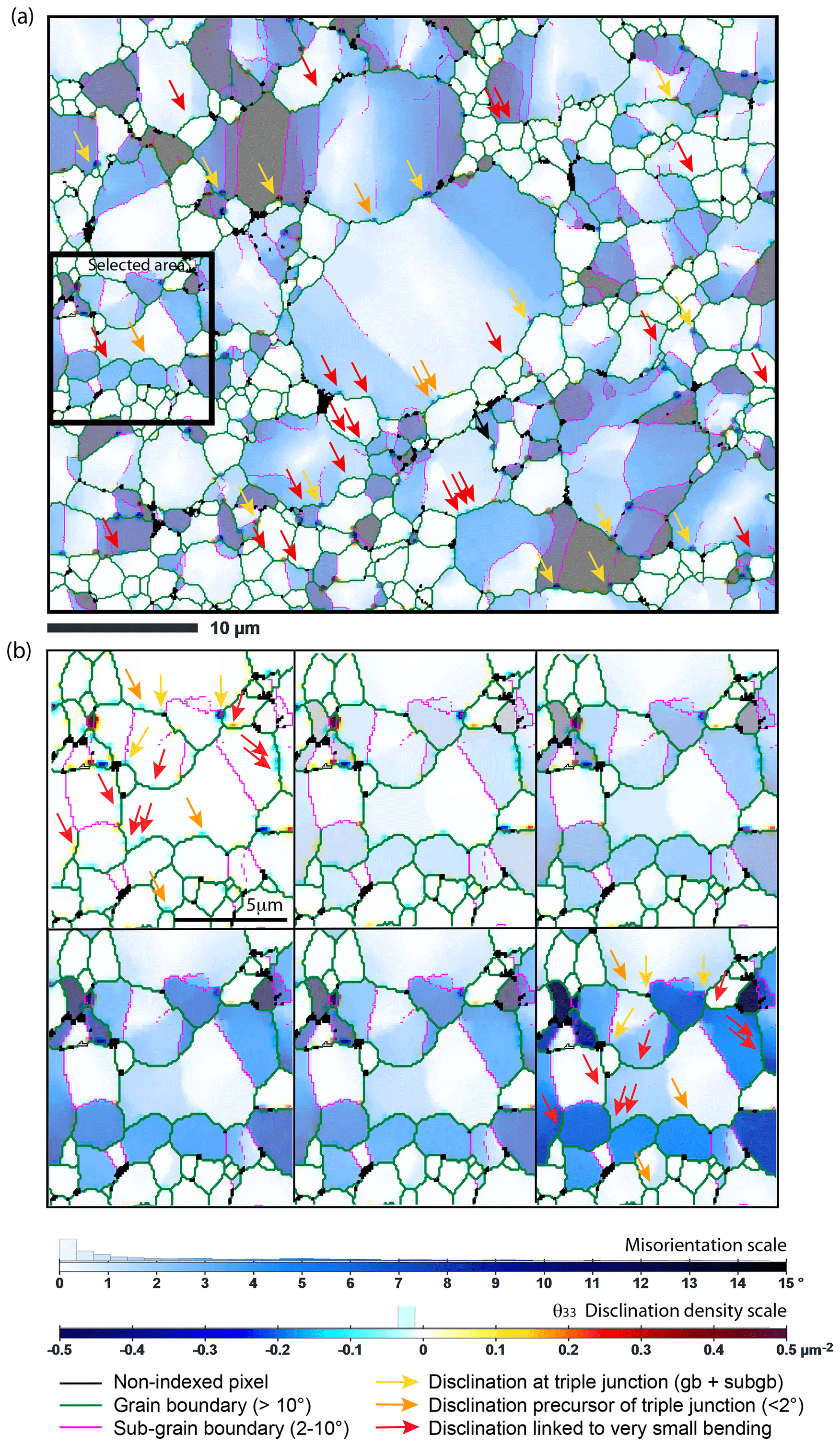
Figure 14 (a) Misorientation maps in sample CMT-16-9 (extracted in the full map) overlaid on the disclination density map (θ₃₃ only). Misorientation in each grain is relative to the center of gravity. (b) Further enlargement of the map in (a) but for different levels of overlay to show the relationship between misorientation from GND and misorientation from disclinations. Three types of disclinations are identified (yellow, orange, and red arrows). See main text for details and Fig. S2.

4.3 Elastic-energy distribution: GND and disclination interactions

To clarify the potential interactions between GND and disclinations, we now present the FDDM simulation predictions using the GND and disclination densities obtained from EBSD maps as inputs. The elastic-energy distribution in the aggregate deformed axially (with 1000 MPa of applied macroscopic compressive stress, as for low-temperature experiments; Thieme et al., 2018; Gasc et al., 2019) is shown in Fig. 15a. The resulting map shows the mechanical incompatibilities coming from elastic anisotropy and different olivine crystallographic orientations in grains for a section of CMT-16-9 (same as in Fig. 14). The stored energy distribution from GND only is shown in Fig. 15b, and that from disclinations is only in Fig. 15c. The energy obtained with both types of defects is finally shown in Fig. 15d. GND and disclinations do not yield the same energy distributions, and they also highlight different areas of the sample aggregate. The GND energy majorly appears concentrated in a few grains around a larger grain size, with a maximum of 400 J m⁻³, while the disclination energy is generally more diffuse in the aggregate, with a few “hotspots” with a maximum around 800 J m⁻³. Moreover, when both defects are simultaneously considered, the energy level and then the distribution is logically controlled by disclinations (Fig. 15d), but several areas display a reduced total energy (blue arrows in Fig. 15d), while in other areas, the energy builds up (pink arrows in Fig. 15d). These maps thus permit the inference of rather complex interactions between GND and disclinations and motivate future analysis.

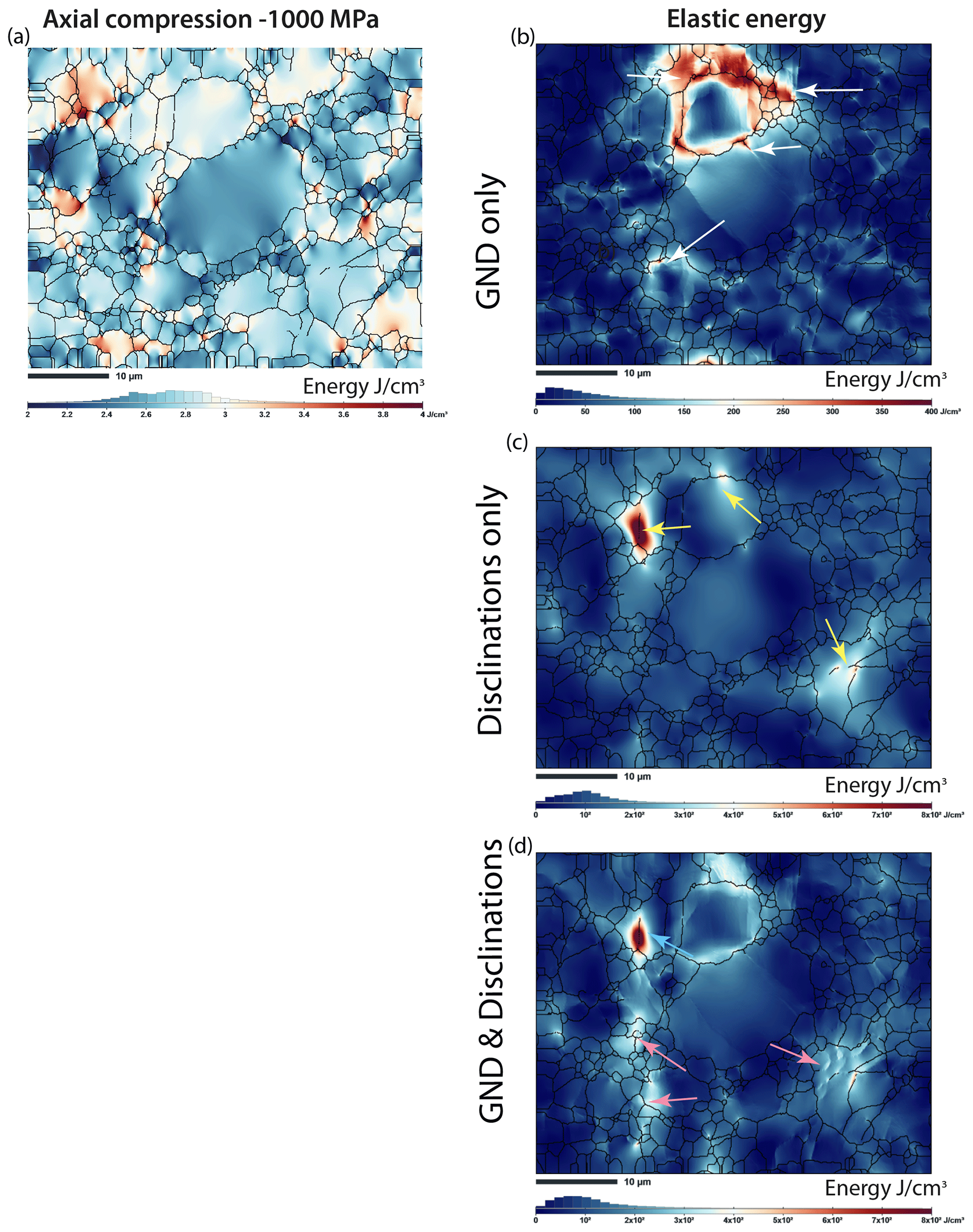
Figure 15 Maps resulting from field dislocation and disclination mechanics (FDDM) simulations of a section of sample CMT-16-9 (a) after axial compression (1000 MPa), designed to reveal mechanical incompatibilities from crystallographic orientation in adjacent olivine grains; (b) with no compression, designed to reveal the action of GND only on internal elastic energy; (c) with disclination only on internal elastic energy; or (d) with both GND and disclination on internal elastic energy.

4.4 Methodological limitations and potential application to natural peridotite specimens

Despite using conventional EBSD and not high-angular-resolution EBSD, the treated EBSD maps presented in this study permit identifying and quantifying new types of defects in olivine (minor GND and disclinations). A logical improvement would be the combination with high-angular-resolution EBSD, based on the transmission Kikuchi diffraction and simulated electron backscatter pattern combined with digital image correlation (e.g., Britton and Wilkinson, 2011; Wallis et al., 2016). However, for none of these three techniques is the size of EBSD maps (e.g., 500 × 500 µm) which can be acquired and treated far smaller than the size of a regular petrological section (e.g., 45 × 30 mm). This also requires significant acquisition time (often > 10 h) and generates large size files. Therefore, the methodology reported in this study must be seen as a complementary technique to locally deciphered mechanisms of deformation since it is not as statistically powerful as conventional EBSD maps on a regular rock section (> 500 grains of mm size). However, this technical limitation is nevertheless going to be improved upon with increasing calculation capacity and decreasing data acquisition time. Another limitation is the exactness of the output values. Since we have only five out of nine components in the Nye tensor, the GND and the disclination densities (three components) are only a partial (a minima) density and will never be absolute values. Thus, potential strain evaluation or stress (after application of Hooke's law) extracted from such data contains only partial values related to the local elastic energy, which is poorly related to what is happening at macroscale (e.g., stress–strain curve of a deformed centimetric sample). Each treated EBSD map must then be interpreted with care when compared to others or regarding its mechanical data.

5 Conclusions

In this paper we report GND and disclination densities in deformed polycrystalline olivine from a broad range of experimental conditions. Based on the new data set, we find that (1) GNDs form not only sub-grain boundaries of mixed character but also a secondary pervasive network; (2) the disclination monopoles and dipoles are observed along grain boundaries in non-deformed and deformed samples; and (3) disclination densities appear independent of bulk stress, strain, or even the temperature of deformation, but the actual values depend on the acquisition step size. Nevertheless, (4) the disclination density is inversely correlated to grain size, suggesting that the action of disclinations compensate the lack of dislocation motions in the smallest grains; (5) detailed observation of selected areas of EBSD maps suggests that disclinations could act as a precursor of GND during the formation of misorientations and (6) could also interact with GND. (7) Even if improvements remain possible regarding reaching dislocation densities and disclination densities independently of the acquisition setup, we have provided a first set of rules to be followed to compare future results. At last, our results support the finding that disclinations act as a plastic deformation mechanism by allowing rotation of a very small crystal volume.