the Creative Commons Attribution 4.0 License.
the Creative Commons Attribution 4.0 License.
 | 28 Feb 2022
Lower mantle geotherms, flux, and power from incorporating new experimental and theoretical constraints on heat transport properties in an inverse model
Anne M. Hofmeister
An inverse method is devised to probe Earth's thermal state without assuming its mineralogy. This constrains thermal conductivity (κ) in the lower mantle (LM) by combining seismologic models of bulk modulus (B) and pressure (P) vs. depth (z) with a new result, ∂ln(κ) ∂P ∼ , and available high temperature (T) data on κ for lengths exceeding millimeters. Considering large samples accounts for the recently revealed dependence of heat transport properties on length scale. Applying separation of variables to seismologic vs. depth isolates changes with T. The resulting LM dT dz depends on and which vary little among dense phases. Because seismic is discontinuous and model dependent ∼ 200 km above the core, unlike the LM, our results are extrapolated through this tiny layer (D′′). Flux and power are calculated from dT dz for cases of high (oxide) and low (silicate) κ. Geotherm calculations are independent of κ, and thus of LM mineralogy, but require specifying a reference temperature at some depth: a wide range is considered. Limitations on deep melting are used to ascertain which of our geotherm, flux, and power curves best represent Earth's interior. Except for an oxide composition with miniscule , the LM heats the core, causing it to melt. Deep heating is attributed to cyclical stresses from > 1000 km daily and monthly fluctuations of the barycenter inside the LM.
- Article
(3297 KB) - Full-text XML
- BibTeX
- EndNote


Heat moves when a temperature (T) difference exists, where the net flow is from hotter to colder regions. This phenomenon is important to Earth because it is dynamic. But as a consequence, the outcome of a laboratory experiment is greatly influenced by the time dependence of the applied heat (e.g., Tye, 1969), which has led to overlooking the length-scale dependence of heat transport and misunderstandings of experimental limitations and uncertainties as well as of microscopic mechanisms (Hofmeister, 2019, 2021). Thermal models in Earth science are particularly affected by these shortcomings, due to wide variations in relevant length scales, temperature, pressure, and material properties, such as transparency to thermal radiation. An improved understanding, based on a new theory and accurate data on mineral heat transport, is described next.
1.1 Recent findings on heat transport properties relevant to mantle studies
One incorrect presumption is that the physical properties representing heat flow (thermal conductivity, κ, or its close relative thermal diffusivity, D) are independent of the distance along the thermal gradient. This static view is inconsistent with Fourier's heat equation, as follows. Its simplest one-dimensional form is
where t = time and z represents the direction of heat flow. Equation (1) holds for temperature changes being sufficiently small that the relevant properties vary negligibly. Dimension analysis of this effectively constant T condition provides
where L is the distance over which heat travels, ζ is a time constant, and u is a characteristic speed. Thermal conductivity likewise depends directly on L because it is proportional to D,
and because the multiplying parameters, density (ρ) and specific heat (cP) at constant pressure (P), are independent of L.
The required length-scale dependence has been masked by experimental limitations, including ubiquitous use of similar sample lengths of > 1 to < 5 mm. Many experiments are steady state, so time and ζ are irrelevant. Other common techniques are periodic, where these oscillations about quasi-equilibrium involve another, different time constant (see, e.g., Tye, 1969; Zhao et al., 2016). The transient technique of laser-flash analysis (LFA), which avoids heat losses from physical contacts (see Vozár and Hohenauer, 2003) and monitors thermal evolution across L with time, has confirmed that D linearly depends on L below about 1 mm for electrical insulators, glasses (Hofmeister, 2019, chap. 7), semi-conductors, metals, and alloys (Hofmeister, 2021). Results (Fig. 1) are consistent with a linear response when L is small, as in Eq. (2).
Misunderstandings also stem from reliance on the historic kinetic theory of gas (KTG) to depict heat transfer in solids. However, heat and matter move together across long expanses in a gas, which is unlike a solid where these motions are decoupled. Furthermore, KTG assumes elastic collisions, through which temperature cannot change. Neither non sequitur is addressed by morphing molecular collisions in a gas into elastic scattering of pseudo-particles denoted as phonons in a solid. Because gas data are collected under negligible T gradients to avoid convection, assuming random fluctuations in all three directions is reasonable and provides formulae mostly compatible with gas data. Yet, the ratios of the transport properties are not correctly described, while the ubiquitous emission of thermal radiation from all states of matter remains unexplained. Accounting for inelasticity in molecular collisions addresses both shortcomings in KTG (Hofmeister, 2019, chap. 5).
Regarding condensed matter, Fourier assumed heat flows into, across, and out of the stationary solid, whereby part of the heat is stored in the elements along the path. The process is diffusion, which is underscored by Fick constructing his formulation after Fourier's.
Fourier defined flux as heat per area per time and realized that
One dimension suffices for discussion since heat flows down the thermal gradient per the second law of thermodynamics. Equation (4) is fundamental: taking its spatial derivative, conserving energy, and simplifying using the definition of Eq. (3) leads to Eq. (1).
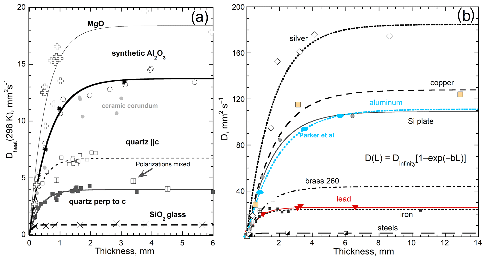
Figure 1Dependence of thermal diffusivity at 298 K on thickness, for various samples, as labeled. Fits are least squares. (a) Insulators with simple compositions. Parallel and perpendicular orientations are shown for quartz. After Hofmeister (2019) – this is the revised and augmented version in Hofmeister (2021). (b) Nearly pure elements and two alloys. At low thickness, the trends are linear and converge. After Hofmeister (2021), with a Creative Commons license.
Experiments and theory show that light is the diffusing entity in solids (Hofmeister et al., 2014; Criss and Hofmeister, 2017), which is real and pure energy. Light, unlike a phonon, crosses interfaces. Attenuation of light across the sample provides the length-scale dependence of Fig. 1. These recent discoveries led to new formulae for the dependence of κ on P and T and the absorption spectra of a material, which were verified against reliable data on κ below 2 GPa (Fig. 2) and on D and κ from a few kelvins to well above ambient T (Hofmeister, 2019, 2021). LFA measurements of D at high T (Fig. 3a), combined with Eq. (3), show that κ above 1000 K is nearly constant for structures or chemical compositions more complex than Al2O3 (Fig. 3b). These advances are used in the present paper to evaluate of thermal conductivity in the lower mantle (LM) while accounting for ambiguities in the temperature and mineralogy for this immense region of the Earth.
1.2 Reliability of available information on lower mantle heat transport
Thermal models are based on transport properties. To achieve high pressures appropriate to the deep Earth, diamond anvil cell (DAC) experiments probe tiny samples. Accurately determining P near 1 atm in devices geared for extreme compression has not been achieved. Hence, results from DAC heat transport experiments are benchmarked against independent measurements of D or κ at ambient P (e.g., Hsieh et al., 2009). However, ambient data are collected from L > 1 mm, which are ∼ 100× larger than sample thicknesses used in DACs. Extrapolation from large to small L was not done and is non-linear (Fig. 1). Very high P studies are difficult, leading to additional problems, as discussed in detail by Hofmeister (2009, 2010b, 2019, 2021). To summarize, large thermal gradients preclude use of Eq. (1) while requiring knowledge of the T dependence of D (or κ) at P, which is the unknown sought. For tiny samples, heat flow is two-dimensional but one-dimensional equations are used. At high T, cooling occurs by ballistic radiation to the surroundings (e.g., to the detector used to ascertain T), which is not addressed in Fourier's description of heat diffusion (conduction). Thermal gradients changing direction during the experiments of McWilliams et al. (2015) and Konôpková et al. (2016) (see figure 13 in Hofmeister, 2021) were not addressed in their analysis. Thermoreflectance methods (e.g., Hsieh et al., 2009) assume the length scale over which heat diffuses, which dictates the results per Eqs. (1) to (4). Low P experiments using ∼ millimeter lengths and other techniques utilized in Fig. 2 lack these difficulties, as discussed in previous work and Sect. 3, and are utilized here.
Importantly, thermal gradients inside Earth are low. Even in the lithosphere, only reaches ∼ 20 K km−1. Thermal transport properties vary little over a few degrees (Fig. 3). Because T varies less than 4 K over L > 5 km inside Earth, its thermal length scale is immense, and so heat transfer therein is always diffusive and isothermal properties are relevant. But in the laboratory, L is ∼ 105 smaller, permitting ballistic (boundary-to-boundary) transport to augment diffusion, as recognized in minerals and rocks by Kanamori et al. (1968) and further documented by Pertermann and Hofmeister (2006), Branlund and Hofmeister (2007), and Merriman et al. (2018). Laser-flash experiments reduce and remove ballistic effects via sample coatings and via models (e.g., Blumm et al., 1997; Hahn et al., 1997). Our large and growing LFA database (e.g., Hofmeister, 2019) and the associated theoretical model are essential to ascertain heat transport at high mantle temperatures.
Seismic models provide velocities and density inside the Earth. Pressure is well constrained, since Earth's mass and moment of inertia provide independent boundary conditions (e.g., Anderson, 2007). Mineralogy is based on comparing laboratory data on minerals to radial models, such as the preliminary earth reference model (PREM) of Dziewonski and Anderson (1981) since radial changes depict average values. Comparison with laboratory studies in a forward-(fitting) approach is used but leads to equivocal results because temperature is not known independently. For the Earth, temperatures are changing, heat is moving, and seismic waves contribute energy to the rocks during their attenuation. Hence, conditions are not adiabatic, as previously assumed in forward-(fitting) models. In addition, minerals vary greatly in possible chemical compositions and structures.
Assessing the lower mantle is particularly uncertain because no rocks have been exhumed from below 670 km. Inclusions in diamonds only indicate P and T conditions when a single inclusion contains multiple phases because most, if not all inclusions, predate their diamond host (Nestola et al., 2017). The inference that lower mantle material is preserved in microdiamonds is based on separated inclusions of (Mg,Fe)O and enstatite (Stachel et al., 2000). The tetragonal garnet phase TAPP (now jeffbenite) once considered to form in the lower mantle is now known to be stable above 13 GPa, i.e., in the transition zone (Nestola et al., 2016).
Evaluating temperatures from seismic models via forward-fitting requires knowledge of the mineralogy (e.g., Cammarono et al., 2003). A thermal model is needed to account for Earth's heat being lost to space (i.e., non-adiabatic gradients). For the lower mantle, a wide range of κ values is possible due to the ambiguities in mineralogical models, even if experimental uncertainties were small. An alternative approach to fitting seismic velocities is needed to better understand this immense region of the thermally evolving Earth.
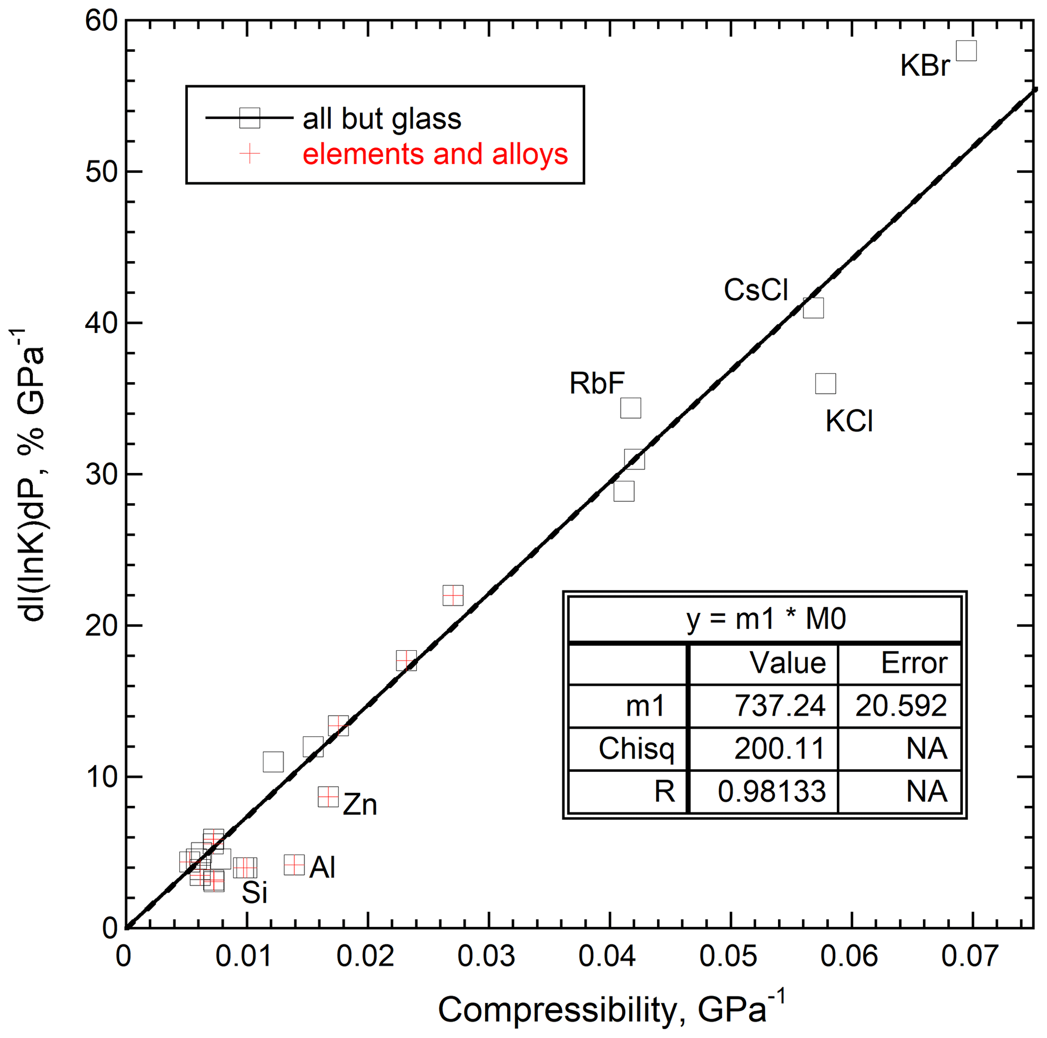
Figure 2Measured pressure derivatives of thermal conductivity as a function of sample compressibility (the inverse of bulk modulus). All data were collected from millimeter-sized samples below 2 GPa. The box lists parameters for a linear fit with no intercept. Metals and Si (red crosses) are included in the fit. KBr exemplifies hydroscopic alkali halides which are soft (bulk moduli < 16 GPa). Details on the 24 heat transport studies of this figure are given in Hofmeister (2021), Table 3. Bulk modulus has been measured many times for the samples and is listed in the compilation of Bass (1995) and several others.
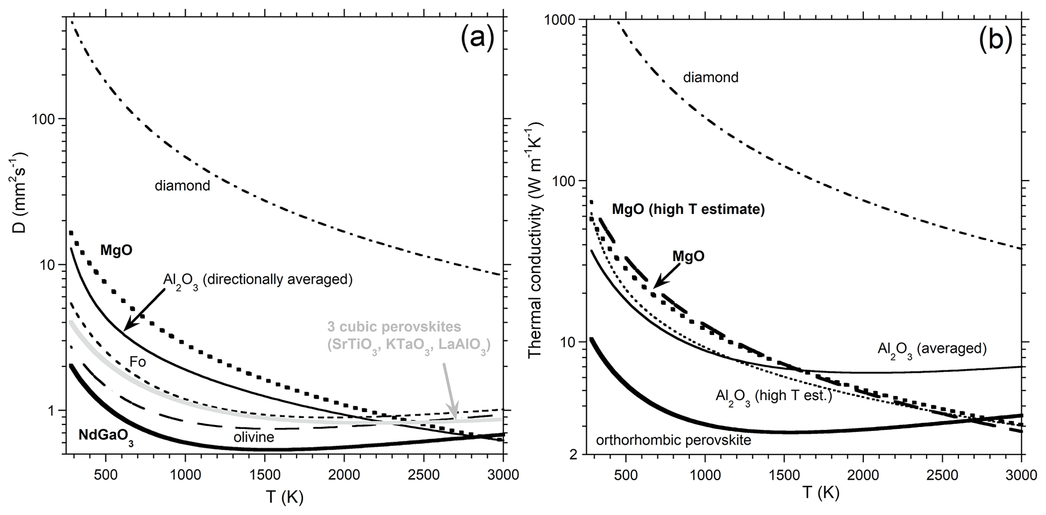
Figure 3Heat transport properties of selected dense solids with a logarithmic y scale. (a) Thermal diffusivity on single crystals from laser-flash analysis, measured up to ∼ 1800 K. Fits using three parameters are shown. Diamond from Hofmeister et al. (2014). Oxides from Hofmeister (2012). Forsterite and olivine are 001 plates (Pertermann and Hofmeister, 2006). Perovskites from Hofmeister (2010a). (b) Thermal conductivity calculated from data on D, cP, and density using Eq. (3). For the oxides, the dotted lines use constant, high-T values for cP and ρ, whereas their other curves use temperature-dependent data. Orthorhombic perovskite is an estimate for a wide range of compositions; see Sect. 3.1.
1.3 Purpose and thesis
In view of limited knowledge of the LM, an analytical inverse approach is used here to decipher its thermal state from a seismic reference model with minimal assumptions. As in previous large-scale mineralogical or thermal studies (e.g., MacDonald, 1959; Anderson, 2007; Murikami et al., 2009; Criss and Hofmeister, 2016), average, radial temperatures are sought to describe Earth's structure, which is reasonably represented as spherical shells. Surface heat flux being remarkably similar for the continental and oceanic crusts, despite the great contrast in their heat-generating elements (e.g., Veiera and Hamza, 2018), points to the radial thermal gradients dominating Earth's thermal state and evolution. The low measured surface emissions of ∼ 60 mW m−2, corresponding to ∼ 100 W km−3 of underlying rock, show that thermal evolution is now slow; i.e., conditions are quasi-steady state. Hence, angular (lateral) motions of heat are unimportant to describing Earth as a whole.
Our mathematical analysis is based on decades of mineral physics efforts which show that (1) pressure derivatives of diverse physical properties vary far less than ambient values do and that, as P climbs, all properties increase more weakly with P. (2) Physical properties at high T behave similarly, as illustrated by the Dulong–Petit limit representing heat capacity at high T. (3) Second-order P or T derivatives of physical properties are small, which means that cross derivatives are small, and so separation of variables reasonably describes many physical properties. Tabulated data on diverse properties and phases (e.g., Anderson and Isaak, 1995; Bass, 1995; Fei, 1995; Knittle, 1995) illustrate these points.
If variables are separable, a property of interest (Υ) follows the form
where f and g are independent, dimensionless functions. Equation (5) describes bulk and shear moduli from diverse elasticity experiments (e.g., Anderson and Isaak, 1995; Bass, 1995). This finding is important to heat transport, as bulk modulus is the prime descriptor of κ(P) per dimensional analysis (e.g., Dugdale and MacDonald, 1955).
For the lower mantle, variations in velocities from available seismic reference models differ negligibly except for the ∼ 200 km above the core (D′′) where variations among studies are small, despite larger uncertainties for this region (see figures in Kennett et al., 1995). Utilizing PREM suffices (see Section 2.1 for further discussion). In the LM, excluding D′′, velocity changes are slow and smooth, leading to interpretation of invariant chemical composition. Since T changes far more slowly with distance in the Earth than in experiments, an isothermal bulk modulus represents the mantle values. The present paper assumes that changes in mineralogy of the LM are secondary, i.e., that the main changes in its seismic radial profile are from P and T, which permits use of Eq. (5). General behavior of bulk moduli for dense materials from both compression and elasticity studies supports this contention.
It is most fortunate that the derivatives are simply described:
where for dense and hard materials compatible with the LM, the constant B′ = is commonly near 4 and is negative and sufficiently small to require very high pressure for its resolution (e.g., Sinogeikin and Bass, 1999; Zha et al., 2000). Results center on because this value corresponds to a harmonic interatomic potential (e.g., Hofmeister, 1993) and anharmonicity links to T, not P, changes (e.g., Wallace, 1972). Most measurements provide as a constant. Although second-order T derivatives exist, these are small (if even resolvable) for hard oxide and silicate minerals, as shown in compilations and more recent work (e.g., Aizawa et al., 2004).
1.4 Synopsis of our novel, analytical inverse approach, and organization of the report
Section 2 shows how to extract the LM temperature gradient () from pressure and depth derivatives of radial seismic reference models by using Eqs. (5) and (6), in an inverse approach. Fitting is not used, which describes familiar, forward modeling. The extraction uses generic values for and , which describes dense phases, including the rock salt and perovskite type structures thought to occur in the deep mantle, to explore the possible range of and its depth dependence. Thus, our thermal model is independent of what phases with what compositions might exist in the LM. The method is new, so details are provided.
Section 3 sets upper and lower bounds on heat transport properties for the LM based on verifiably accurate methods. We derive a simple formula for from Fourier's heat equation, which confirms that the result of Hofmeister (2021) is an identity. The sole parameter in the identity (other than BT and P) appears be a constant, as suggested in Fig. 2 and independently by previous work (e.g., Chopelas and Boehler, 1992). The resulting bounds on κ(T,z) for the LM, combined with derived from PREM (Sect. 2), provide flux and power across the LM, without assuming its mineralogy.
Section 4 constructs geotherms using a reference temperature at a shallow level that avoids melting of a peridotite composition anywhere in the LM. These geotherms are independent of κ. Then, we ascertain which of our geotherms, fluxes, and powers are compatible with additional constraints, such as phase equilibria and latent heat of melting.
Our inverse model, which is based on radial seismic changes and high T and P behavior common to dense phases, indicates that the LM has a heat source which is warming the outer core, while causing the inner core to melt. Possible heat sources are discussed in Sect. 5, along with implications of our results.
2.1 Features of PREM
Seismic reference models represent Earth's average interior; i.e., they are radial. Aspherical images of the Earth's internal structure are represented as perturbations to a reference mode (e.g., Ritzwoller and Lavely, 1995).
Reference model results are displayed as the fairly smooth functions of velocities, density, and pressure as a function of depth (z) or radius (s), or similarly as plots of bulk and shear moduli, the quantities of which are also fairly smooth, being derived from ρ and the two velocities. Seismic discontinuities are present as kinks, most of which are small in these typical representations. In contrast, large jumps dominate plots of derivatives of variables vs. depth (Fig. 4). Hence, this paper makes use of the derivatives.
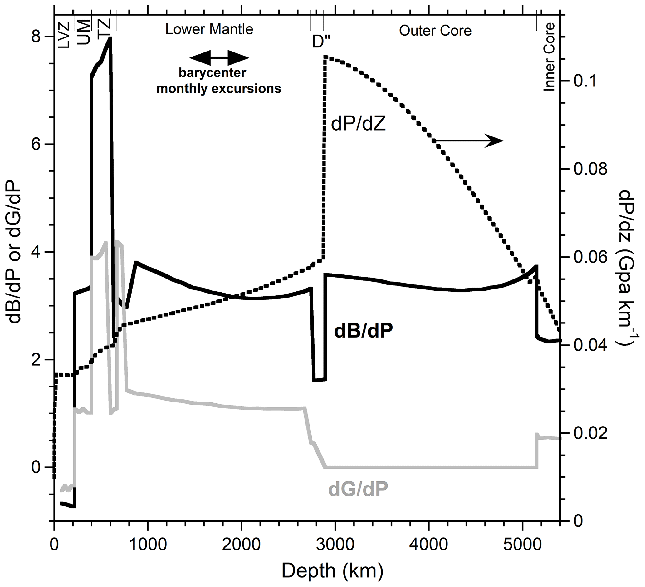
Figure 4Derivatives from the seismologic model PREM (Dziewonski and Anderson, 1981) as a function of depth. Variables as tabulated by Anderson (2007), from which we calculated the pressure derivatives of the bulk (black) and shear moduli (grey) as well as the depth derivative of pressure (dots).
Taking derivatives accentuates differences, as this mathematical operation is the converse of integration, which averages and smooths. The pattern exhibited by velocity derivatives (not shown) is similar to moduli derivatives, whereas the density derivative (not shown) is relatively smooth, more like the pressure derivative, and so the depiction of Fig. 4 is inherent to PREM.
Smooth and continuous describes the lower mantle but only between depths of 871 and 2741 km (Fig. 4). Importantly, other reference models such as Ak135 differ negligibly from PREM velocities in this restricted region (see Fig. 12 in Kennett et al., 1995). Our approach (below) applies to continuous functions only, so PREM suffices to represent all reference models of this volumetrically immense region. However, D′′, where seismic models differ, cannot be quantitatively analyzed. We can only extrapolate into this tiny shell. For brevity, “lower mantle” or “LM” refers to its central region from 871 to 2741 km only, unless specified otherwise. Extrapolation of results for the LM into the underlying D′′ layer and up to 671 km, which defines the transition zone (TZ), is discussed in Sects. 4 and 5.
2.2 Separation of variables
The geothermal gradient is defined by
PREM provides the input quantity (Fig. 4). PREM values for B and as a function of depth are affected by both compression and heating of the minerals inside the LM. Our goal is to utilize available data to distinguish the effects of P and T on B from PREM. This is possible through separation of variables and decades of data acquisition.
Equation (6) provides the input for . Because an inverse approach is being used, we consider values compatible with many dense phases, oxides, and silicates. The changes (differences) below z = 871 km are of interest, so the value of at 871 km serves as a reference point. This approach links B′ and B′′, as shown graphically in Fig. 5. Hence, obtaining thermal gradients from PREM via Eq. (7) requires some estimates of and but not of . This is understood by considering two end-member cases.
The case B′′ = 0 for the lower mantle sets an upper limit since B′′ is not positive. If this commonly used limit (e.g., Knittle, 1995) applies to the LM, then with depth solely results from compression and thus is invariant (horizontal dashed–dotted line in Fig. 5). Consequently, rising temperature causes the linear decrease in PREM with z immediately below 871 km under separation of variables. For the second case, we consider B′′ = −0.015 GPa−1, which reproduces the decrease in PREM with z below 871 km. With this match, changes in B of PREM solely result from compression; i.e., T is constant for z slightly below 871 km. Hence, B′′ between 0 and −0.015 GPa−1 depicts a LM that is both compressing and warming below 871 km, whereas B′′ > −0.015 GPa−1 depicts a cooling and compressing LM just below 871 km. This case is not shown because T in the outermost layers of the Earth increases with depth, and so the top of the LM should behave likewise.
Once z reaches 1300 km, PREM curves have become rather flat, but as z increases further, deeper than ∼ 2200 km, PREM curves take on a positive slope with z, which is linear just below 2741 km. The broad minimum near 2000 km suggests that a maximum temperature may exist in the LM, where its manifestation depends on mantle values of and (discussed below). The positive slope in PREM curves at great depths, assuming that Eq. (6) represents the LM, shows that its deepest extent is shedding its heat downwards while compressing, discussed further in Sect. 4.
The above findings are general. Here we emphasize that following the discovery of heat generation by radionuclides, it was recognized that Earth may be heating up rather than undergoing progressive cooling. This question was considered in some remarkable papers (e,g., MacDonald, 1959). Notably, Takeuechi et al. (1967) devoted an entire chapter of their book to this subject.
Importantly, temperature differences from the starting point at 871 km are germane. Consequently, the input for in Eq. (7) is the PREM curve less a line for the P response of B, i.e., Eq. (6). Figure 5 shows the two end-member cases, discussed above, and one intermediate case. These three examples show that B′ is controlled by the choice of B′′, in order to match the starting point at 871 km. The range of values of 3.8 to 4.3 is compatible with mineral data (e.g., Knittle, 1995), with 4 being the harmonic value (Hofmeister, 1993).
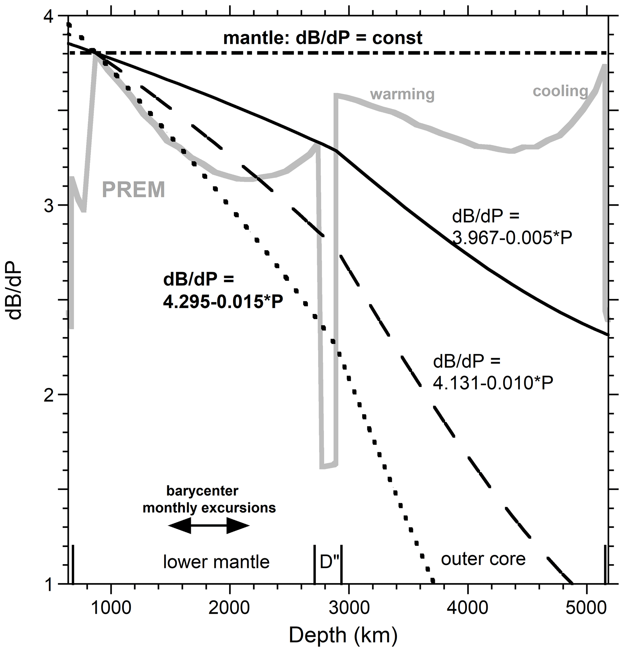
Figure 5Construction of possible curves for the depth response of the P component of mantle at 871 km and deeper. The edges of the transition zone and inner core define the x axis. Discontinuities shallower than 871 km and in D′′ are not addressed in our approach. If is small, near 0, then PREM indicates that warming first occurs as z increases but at greater depths temperatures decrease. This behavior describes the LM and outer core.
2.3 Constraints on and from elasticity and volumetric measurements of diverse phases
Regarding the thermal input parameter, equals −0.023 GPa K−1 from the average of four experiments on MgO (compiled by Bass, 1995) and is only slightly larger in magnitude, −0.029 GPa K−1, for MgSiO3 with the perovskite structure (Aizawa et al., 2004), now known as bridgmanite. A large range of values is possible, per Aizawa et al. (2004) and work cited therein. More importantly, uncertainties are high while similar values are observed for corundum, spinel, five compositions of olivine, orthopyroxene, zircon, five garnets, seven other oxides, and four metals, whereas framework silicates, diamond, and alkali halides have near −0.01 GPa K−1 (Bass, 1995; Anderson and Isaak, 1995).
An input value of −0.026 GPa K−1 is used, the average of which is within reported experimental uncertainty of measurements of LM candidate minerals and moreover describes dense silicates and oxides in general. Because is inversely proportional to , the effect of varying this parameter on the results is easily ascertained. In contrast, a non-linear response is associated with B′′, since a difference with PREM is involved and PREM curves are non-linear with depth (Figs. 4 and 5). Hence, possible B′′ values are the focus.
From the compilation of Bass (1995), B′′ is positive for silica glass and near 0 for MgAl2O4 spinel, which is also disordered. Otherwise, B′′ for oxides and silicates ranges from −0.03 to −1.6 GPa−1. The largest magnitude depicts orthopyroxene, which has unusually high B′ as well. For bridgmanite, B′′ was not resolved even at compression to 155 GPa (Dorfman et al., 2013), consistent with incompressibility of high-pressure, dense phases. Aluminum being present makes no difference (Zhu et al., 2020). However, ubiquitous use of the Birch–Murnaghan equation of state, which involves trade-offs between B and B′ (see, e.g., Knittle, 1995), prevents resolution of B′′ for these stiff structures. Polynomial fits are needed to ascertain B′′.
Many studies exist of MgO, but some ambiguity exists because elasticity data are fit to a polynomial in pressure, whereas volumetric data are analyzed using an equation of state, which is a general formulation for the P and T dependence of volume (V). The second-order polynomial coefficient for B(P) is . To make sure this convention (i.e., Eq. 6) was used, original studies were consulted. Elasticity measurements of MgO by Sinogeikin and Bass (1999) provide B′′ = −0.04 ± 0.02 GPa−1. The X-ray diffraction study of Yoneda (1990) is consistent with the range of 0 to −0.029 GPa−1. Zha et al. (2000) reached the highest pressures and found that the null value reasonably represents elasticity and volumetric data combined. For the dense LM, B′′ is small. Again, B′ = 4 and negligible B′′ describes a harmonic solid (e.g., Hofmeister, 1993). We consider 0 to −0.02 GPa−1, mostly in steps of 0.0025 GPa−1, to calculate from Eq. (7).
2.4 Thermal gradients from 871 to 2741 km
Thermal gradients are shown in Fig. 6, with an example of a fit to B′′ = −0.005 GPa−1. The sign convention used here is based on flow from a central source (s = 0) moving outwards. All curves are well represented by third-order polynomials (Table 1) with similarly high residuals. Fits can be scaled to address variations from an input value of −0.026 GPa K−1. Constrains on are covered in Sect. 4.

Figure 6Dependence of thermal gradients from PREM (black symbols) on depth and the choice of for LM material. Fits are in color, where the inset lists coefficients for B′′ = −0.005 GPa−1, which has a typical residual. For positive gradients, T increases inwards.
Table 1Polynomial curve fits to the thermal gradient in kelvin per kilometer (K km−1), with parameters for the geotherm and power curves.
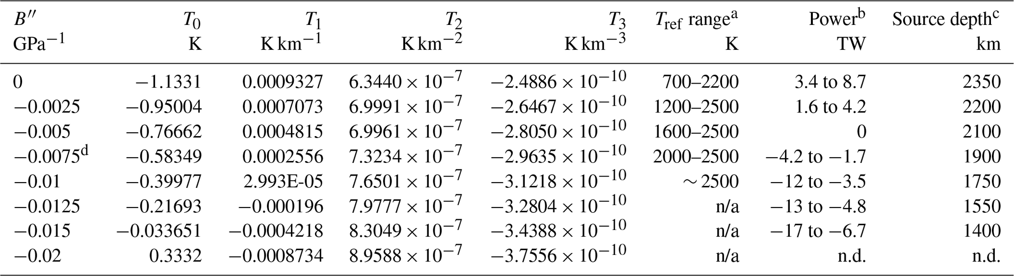
The polynomial for is . n/a: not applicable because large leads to unsupportable melting that occurs near 670 km. n.d.: not determined. a These values satisfy the criteria that the LM is not melted and that the outer core melts above 2750 K as measured for the Fe–S system (see text). b Range at 2741 km from estimates of low and high κ. Power at the core mantle boundary (CMB) is lower, by about 1 TW. Positive sign indicates heat flow from the core into the LM, discussed below. c From the broad maximum in power which is nearly the same for low and high κ. d Most likely to represent the LM; see text.
3.1 Dependence of thermal diffusivity on temperature
Three-parameter fits describe measurements of thermal diffusivity for diverse solids above room temperature up nearly to melting that are neither affected by physical contact losses nor by spurious radiative transfer gains:
The fitting coefficient G is near unity and H is small (Hofmeister et al., 2014). When H = 0, the parameter F* =F(298)G on the right-hand side equals D at 298 K. The general applicability of these formulae has been established by additional measurements now encompassing over 200 substances (Merriman et al., 2018; Hofmeister, 2019). Equation (8) represents sample thickness L > 1 mm, i.e., bulk samples, and high temperatures and thus is appropriate to the mantle.
Examples of D(T) for dense phases are shown in Fig. 3. Generally, H is quite small, ∼ 0.0002 mm2 s−1 K−1, but is essential to represent high-temperature behavior (T > 1200 K) of structures involving unit cell formulae more complex than Al2O3. For simple materials such as MgO and alkali halides occupying the cubic B1 and B2 structures, H = 0 within uncertainty. However, Si with the diamond structure has non-negligible H when impurities are present, whereas graphite, which has a more complicated anisotropic structure and is generally impure, has a substantial H term (Hofmeister, 2019, chap. 7). LFA data on glasses show that large H is commonly associated with high Fe cation content (e.g., Sehlke et al., 2020). These findings point to absorption bands above ∼ 1000 cm−1 and into the visible region being associated with the HT term. To provide H when LFA data on (MgxFe1−x)O are not available, we consider corundum, rather than MgO, to represent an oxide-rich lower mantle. For a silicate LM, systematic behavior of orthorhombic and cubic perovskites with various chemical compositions (Hofmeister, 2010a) is considered. The average D from the three orientations of NdGaO3 is used to compute the T dependence of D for orthorhombic perovskite, since this agrees with D near 298 K for unoriented MgSiO3 from Osako and Ito (1991). A periodic technique was used, and their sample was polycrystalline. Contact losses are more important than ballistic gains, because the latter is reduced by physical scattering between grains. Hence, D(T) for NdGaO3 in Fig. 3a represents a minimum for a complex silicate phase in the LM.
Differences among dense silicates at high temperature are not large: this is the basis of D = 1 mm2 s−1 being commonly used in geophysical models. Near independence of D from T for complex solids at high T considerably simplifies calculations (below).
3.2 Dependence of thermal conductivity on temperature
Figure 3b shows examples of κ(T) calculated from Eq. (3). For MgO and Al2O3, cP and ρ as a function of T are well constrained even at high T (e.g., Ditmars et al., 1982; Fiquet et al., 1997; Chase, 1998). Heat capacity data on MgSiO3 perovskite (Akaogi and Ito, 1993) are limited to near-ambient T due to back-conversion problems. Using a model to extrapolate cP is unnecessary, due to uncertainties in D(T) for silicate perovskite. Since D varies more strongly with T compared to cP and ρ, which moreover respond in opposite directions during heating, ambient values are used to estimate κ(T) for a silicate perovskite mantle. To ascertain the uncertainty in this approach, analogous computations were made for κ(T) of periclase and corundum. Accurate and estimated trends for MgO differ little (Fig. 3b), but the Al2O3 estimate is significantly steeper with T than using exact values in Eq. (3). Corundum D(T) is very flat and is better fit to a polynomial than to Eq. (8), so the discrepancy is likely due to extrapolation beyond the temperatures actually measured. Another factor is that the T variations of both D and κ with T are weak when the corresponding ambient values are low, as is indicated in Eq. (9) and evident in Fig. 3. Thermal conductivity of other silicates depends similarly on T as our estimate for perovskite (for examples, see Hofmeister et al., 2014, and references therein).
Therefore, we estimate high-T mantle thermal conductivity in terms of constant, limiting values. For an insulating silicate LM, κ is taken as 2.7 W m−1 K−1, whereas for a thermally conductive oxide LM, κ is taken as 7 W m−1 K−1. The generic value of D used in geophysical models corresponds to ∼ 3.5 W m−1 K−1.
3.3 Dependence of thermal conductivity on pressure
Many formulae have been proposed for P derivatives of transport properties, based on dimensional analysis. An exact thermodynamic relationship,
was derived and confirmed using reliable available data on 20 different homogeneous solids at pressures up to 2 GPa (Hofmeister, 2021). Equation (9) excludes a typographic error in the earlier report. The physical properties, other than κ, are part of the equation of state (EOS). Thermal expansivity is defined by
Compressibility (, the bulk modulus) is defined by
The dimensionless Anderson–Grüneisen parameter (δT) describes the opposing effects of T and P on V,
while clearly showing that the efficiency of expansion and compression for any given solid is related. Hence, the far-right-hand side (RHS) of Eq. (9) describes how temperature components of the EOS, not just pressure components, regulate changes in heat conduction during compression.
3.3.1 Derivation of from Fourier's equation
Due to the importance of compression to mantle heat transfer, we explain why Eq. (9) is exact. The original derivation considered diffusion of thermal radiation. A simpler approach is covered here.
Since ℑ is independent of pressure in experiments, taking the P derivative of its definition (Eq. 4) suffices to relate to EOS parameters. The algebra is simple and not specified here. However, one must recognize that a negative temperature gradient () is associated with positive signs for ℑ and κ in Eq. (4). But Eq. (10) defining thermal expansivity is a scalar quantity, being based on volume, which has no direction. A positive sign for α, typical of most materials, requires the thermal gradient and its inverse, , to be positive in an isotropic solid. In contrast, heat flow has a well-defined direction from some origin and so is a vector quantity. Maintaining consistent signs for both κ and α during algebraic manipulations after differentiation of Fourier's equation leads to Eq. (9).
3.3.2 Experimental validation
The hot wire/hot strip and Angstrom techniques accurately measure thermal transport in metallic samples at low P (< 2 GPa) and low T (< 1000 K) since metal–metal contact losses are low and ballistic radiative transfer gains are negligible (e.g., Andersson and Bäckström, 1986; Jacobsson and Sundqvist, 1988). Moreover, use of standard L near millimeters in piston–cylinder and multi-anvil apparatuses permits direct comparison of results on diverse materials. Reliable data for insulators at high P over millimeter length scales have been obtained near 298 K using the hot strip/hot wire or Angstrom methods (e.g., Andersson, 1985; Osako et al., 2004). Samples are single crystals, glasses, and disks of fine-grained soft powder (alkali halides) that were compacted prior to study. Unlike metals, systematic errors exist due to interface thermal resistance and ballistic transfer, but taking a logarithmic pressure derivative minimizes these problems. Low-pressure transport property measurements and EOS results of over 20 solids, mainly from elasticity data, are summarized in Table 3 of Hofmeister (2021). The response of thermal conductivity to compression (Fig. 2) points to δ = 7 at ambient conditions representing the average for silicates, oxides, metals, alloys, and alkali halides.
Further verification is provided by a well-studied material with a special, negative sign of thermal expansivity. A negative sign for pressure response for thermal conductivity is expected and was indeed observed for silica glass by Andersson and Dzhavadov (1992) and Katsura (1993). Consistency with Eqs. (9) to (12) is demonstrated, since fused silica also has uncommonly positive (Spinner, 1956).
3.3.3 Previous EOS evidence for nearly constant δT
Chopelas and Boehler (1992) constrained mantle values of δ from 5 to 6 for metals, oxides, and alkali halides by assessing thermal expansivity at high pressure and temperature. Anderson et al. (1992) argued for an ambient value δ0 = 6.5 and a weak volume dependence. The focus of these studies, along with Helffrick (2017), who further modified the V dependence, is the effect of compression on α.
Larger δ0 = 7 was obtained from Fig. 2, which compares measurements of ∂κ/∂T to 1/B for the same types of solids. Hofmeister (2021) calculated δ0 from temperature derivatives of bulk moduli, which are more accurate than P (or V) derivatives of α for several reasons. (1) Elasticity measurements determine as a first derivative and so are more accurate than x-ray diffraction (XRD) studies which determine as well as as second derivatives. (2) Linear dependence of B on T exists over a wide range of temperatures (e.g., Anderson and Isaak, 1995), which simplifies establishing this parameter and reduces its uncertainty. (3) Because B is large in magnitude whereas α is small, derivatives of B are easier to determine accurately. Average δ0 = 7 obtained in Fig. 2 better agrees with the EOS study of Anderson et al. (1992) because they included elasticity data in their assessment. (4) Data on thermal expansivity at pressure from XRD methods give α as an average over the temperature ranges explored, which makes this approach to P derivatives of α very uncertain. High uncertainty in α, let alone its P derivative, is evident in the compilation of Fei (1995).
Pressure-independent δ is consistent with separation of variables describing the bulk modulus, i.e., if
Then from the RHS of Eq. (12) follows
Equation (14) equals 0 when and is small otherwise. Equation (14) suggests that δ is a constant on the order of 4, the value of which for B′ constitutes the simple Murnaghan EOS.
Similarly exploring the middle term of Eq. (12) indicates that δ also weakly depends on temperature when thermal expansivity is described by separation of variables. Constant δ is thus a reasonable first-order approximation. Exact evaluation is difficult due to the generally small sizes of all derivatives, limitations of a polynomial representation, and assumptions underlying the forms for the EOS. Compressible alkali halides are very important for this endeavor but are hydroscopic, easily deformed, and transparent in the infrared as single crystals.
3.3.4 Lower and upper bounds for thermal conductivity in the LM
The pressure (or depth) dependence of κ in the LM is much weaker for perovskites than oxides (Fig. 7), assuming δ0 = 7. Corundum and perovskite have similar bulk moduli, so their different curves in Fig. 7 relate to relative efficiency of heat transfer at high T only.
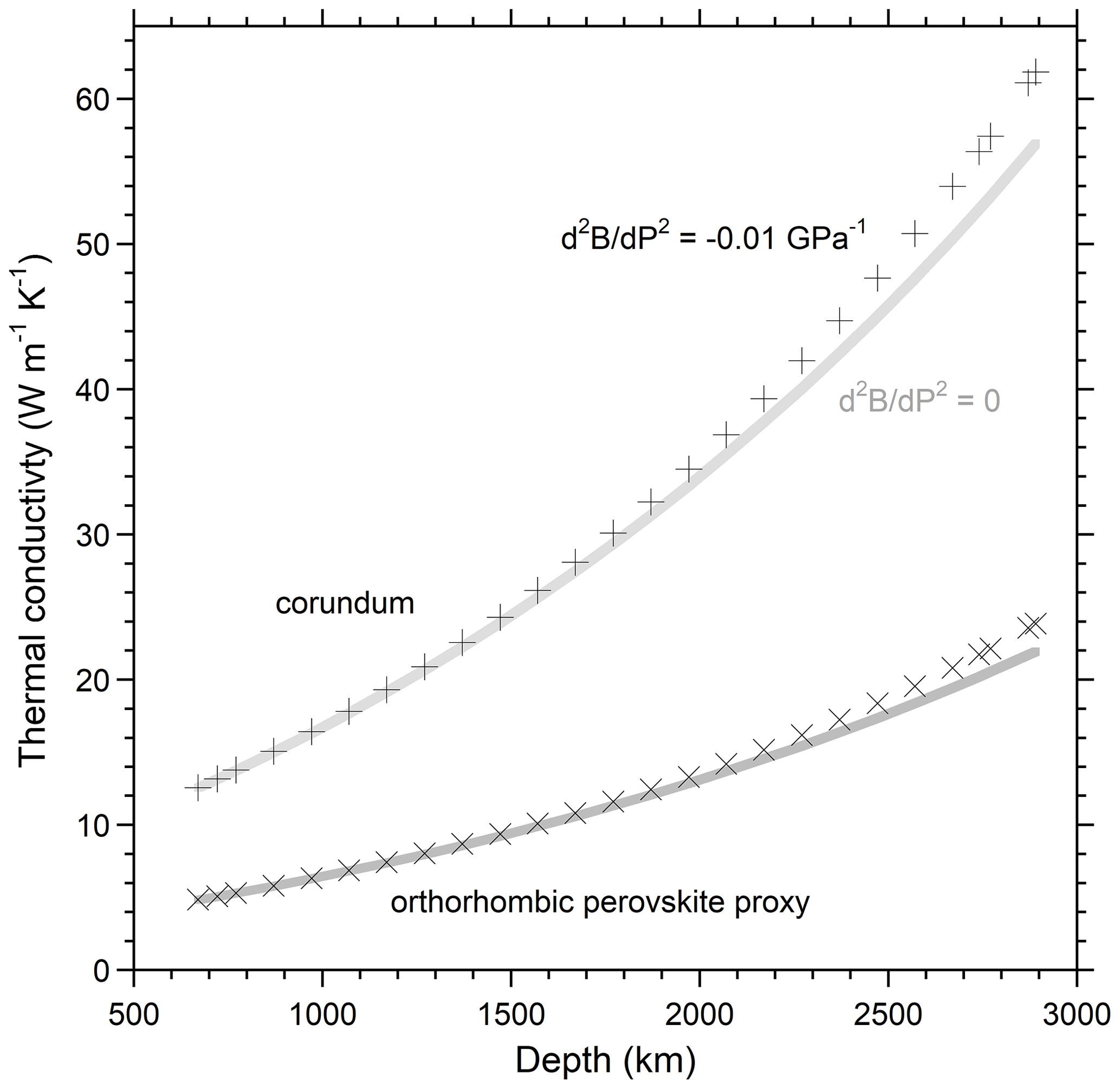
Figure 7Thermal conductivity in the lower mantle for oxide and silicate perovskite compositions assuming temperature independence and using Eq. (9) with δ = 7. Solid curves are computed for B′′ = 0. Symbols utilize larger magnitude B′′ than likely exists, given the results from PREM, but even this makes little difference.
Pure MgO would have lower κ than Al2O3 with depth due to T increasing beyond 1500 K (Fig. 3b) but would have higher κ with depth due to P increasing. For this reason, corundum, which has the same κ as periclase at 1500 K, is used to represent an oxide lower mantle (Fig. 7).
Calculations of geotherms, flux, and power from 871 to 2471 km are presented here, which are extrapolated through D′′. Comparison is made with possible melting temperatures to eliminate cases unlikely to represent Earth's interior. The limiting case of B′′ = 0 is unexpected but is useful for comparisons. Importantly, our geotherms do not utilize data on thermal conductivity and thus are essentially independent of mineralogy. In contrast, flux and power are independent of the reference temperature, but use κ and thus are affected by LM mineralogy. However, as κ varies little at high T (Fig. 3), only the proportion of complex silicates to simple oxides matters.
4.1 Calculation of temperatures across the lower mantle from PREM and a reference point
Geotherms are calculated by integrating the thermal gradients (Fig. 6) which were obtained from PREM, from 871 km downwards, using various B′′ values (Table 1). Results (Fig. 8) consider three values for the 871 km reference temperature (Tref) representing the top of the lower mantle. The minimum Tref of 1500 K is based on temperatures for basalt extruding at the surface (e.g., Falloon et al., 2008), whereas the maximum Tref of 2500 K is based on dry melting of peridotite at 670 km (Zhang and Herzberg, 1994). The intermediate (Tref = 2000 K) corresponds to Takahashi's (1986) melting curve of peridotite at ∼ 410 km, which probably involved tiny amounts of moisture, based on sensitivity of melting to hydration.
All geotherms (Fig. 8) are flat near 871 km, due to PREM derivatives being linear for the shallowest LM (Fig. 6). Thus, the inverse method suggests that temperatures change little from 871 km up to the shallower depth of the 671 km seismic discontinuity. Chemical composition could be changing near 670 km, as descending slabs are resolved from earthquakes down to these depths but not below (summary figures are in Hofmeister, 2020, chap. 7, and in Hofmeister et al., 2022).
Regarding the base of the LM, the geotherms smoothly decrease with depth. Extrapolation of LM results from 2741 to 2891 km presumes similar bulk moduli derivatives for D′′ and the LM. Although this seems unlikely, since reaction with core material is possible, discontinuities at these depths preclude robust analysis (Sect. 2), and modeled velocities in this region are less certain than in the LM (e.g., Kennett et al., 1995). But, as discussed in Sect. 2.3, as evidenced by compilations and recent work, derivatives of B vary little with structure, composition, and bond type.
Melting curves of Fe–S and Fe–Ni–S systems (Chudinovskikh and Boehler, 2007; Morard et al., 2011; Mori et al., 2017) set a minimum of ∼ 2750 K at 2891 km, whereas peridotite melting (Fiquet et al., 2010) sets a maximum near 4100 K (Fig. 8). Only for the combination of the highest Tref and the limiting case of B′′ = 0 is peridotite melting reached. Many, but not all, geotherms exceed the Fe–S eutectic. For example, if Tref = 2000 K, then must be smaller than 0.0075 GPa−1. Table 1 lists the range of reference temperatures consistent with the above-mentioned phase equilibria for each B′′ value considered. Only for the hottest possible Tref = 2500 K can B′′ reach −0.01 GPa−1. Small second derivatives are consistent with difficulty in resolving these in experiments on dense materials, unless extreme pressures are reached (see Zha et al., 2000) and polynomial fits are used (Sect. 2.3).
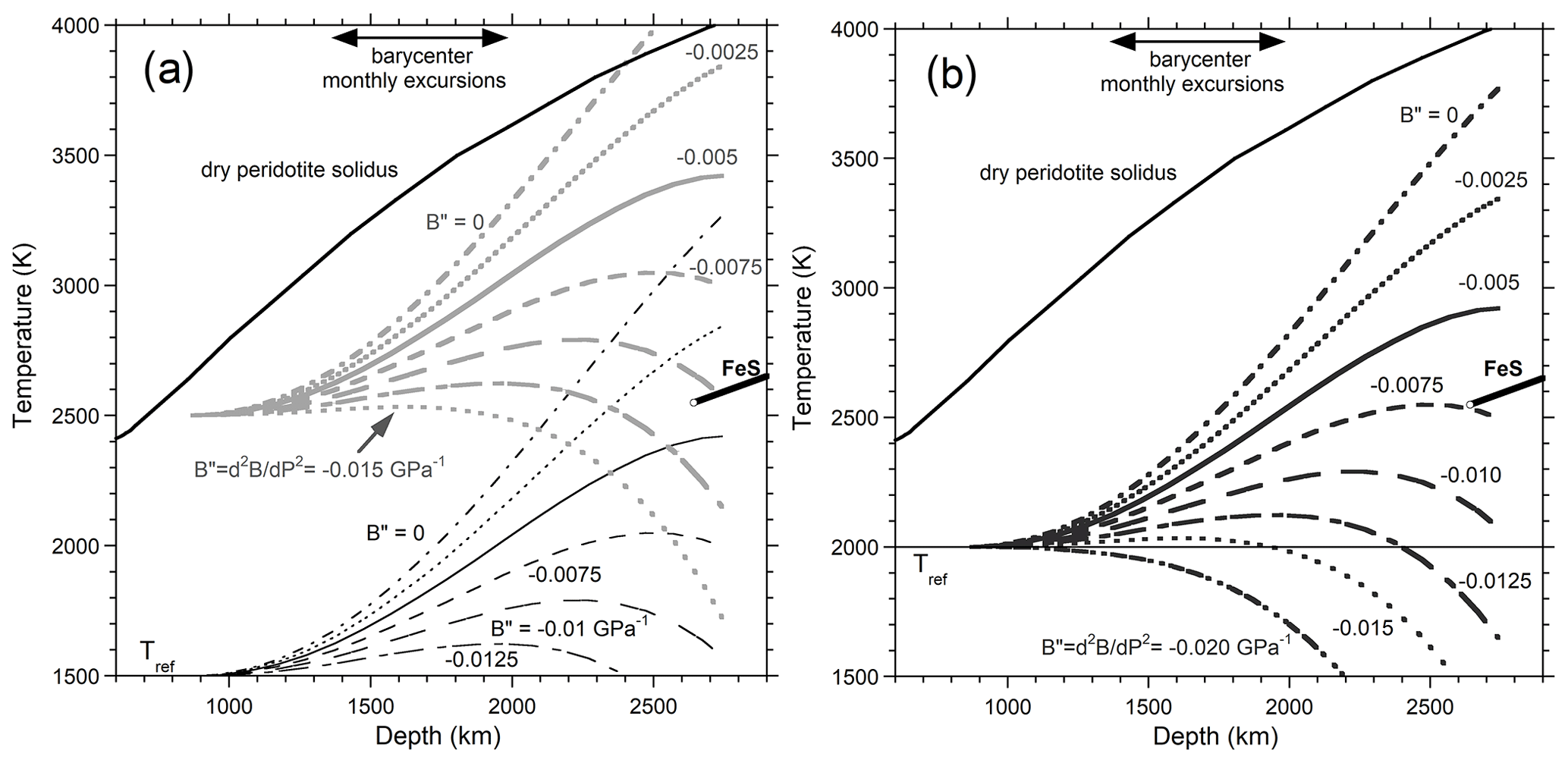
Figure 8Families of geotherms for possible values of second P derivatives of LM bulk modulus and three different starting temperatures at 871 km. All curves use the T derivative of B for silicate perovskite from Aizawa et al. (2004). For the dry peridotite solidus, results of Zhang and Herzberg (1994) are merged with high P data or Fiquet (2010). The thick black line is the eutectic melting curve of the Fe–S system (e.g., Morard et al., 2017).
Irrespective of the temperature values, the shape of the geotherms require a thermal maximum inside the lower mantle. For large magnitudes of B′′, a maximum is indicated roughly near 670 km or slightly shallower. For the smallest , the maximum T in the lower mantle is reached at its interface with the core. In all cases consistent with phase equilibria, maximum LM temperatures are reached for z below 2200 km. Thus, from analyzing PREM curves, LM temperatures climb inwards for most cases considered. A heat source located in the LM is supported by flux and power calculations, below.
Altering our input value for from −0.026 GPa K−1 will either expand or contract the splayed patterns of Fig. 8, which rest on thermal gradients of Fig. 6 obtained from Eq. (7). Comparison of such revised curves with phase equilibria would then change the ranges of B′′ and Tref that avoid melting in the LM while allowing melting in the core (Table 1, RHS), resulting in quite similar shapes. Thus, geotherms from PREM are robust, given the subsidiary information on melting relations, whereas the specific input values are interdependent. The shapes of the geotherms are compatible with the process of heat diffusion, i.e., thermal conduction, even though the calculations (depicted in Table 1 and Figs. 6 and 8) did not incorporate thermal conductivity values.
4.2 Calculation of flux across the lower mantle from PREM and κ
Flux, defined by Eq. (4), describes spherical geometry for radially changing T. Temperature values are not needed to compute the amount of heat being moved inside and across the LM, when κ only weakly depends on T. The gradients of Fig. 6 and Table 1 lead to families of flux vs. depth curves which depend on B′′ values for each of low and high κ. The sign convention used here portrays heat from the center of a sphere moving outwards.
All cases (Fig. 9) provide a broad peak for ℑ across the lower mantle. For comparison, surface flux values are larger, averaging ∼ 60 mW m−2 for either crust (Veiera and Hamza, 2018). The height of the peak in ℑ increases as B′′ approaches its null limit. Only for this limiting case (B′′ = 0) is flux within D′′ large and positive, the behavior of which signifies that heat emitted from the core contributes to the flux in D′′ and at large z in the LM. For the next larger value of B′′, flux near D′′ is positive but near zero. Thus, the vast majority of our calculations point to a lower mantle source whose heat is being shed to its adjacent layers. Section 4.3 provides further discussion.
Note that the curvature and a maximum in ℑ are inherent to PREM (Figs. 4 to 6; Sect. 2.3). The increase in thermal conductivity with P serves to flatten these curves at great depths near the outer core and, importantly, means that the efficiency of heat conduction increases with depth. Consequently, heat from a source deep in the Earth is conveyed more readily inwards than outwards.
How much heat is carried depends on the material, i.e., on the high-T value at ambient pressure. Our model (Fig. 7) rests on heat transport values that are established via measurements. The thermal response at modest temperatures (< 2000 K) of any given material is largely controlled by infrared fundamentals and near-IR overtones, whose frequencies overlap with the associated blackbody curve (Hofmeister, 2019, chap. 11). We have not accounted for electronic transitions of Fe2+ augmenting heat transfer significantly above ∼ 1000 K, as observed in various glasses (Sehlke et al., 2020, and references therein), since the chemical composition of the LM is not known. The purpose of this paper is to ascertain Earth's thermal state with minimal assumptions and input parameters. As accuracy is not possible given the scant definitive information on LM mineralogy, such as samples, salient features not affected by the details are pursued here.
Nonetheless, enhancements in thermal conductivity with depth would raise the flux near 2471 km and straighten the curves, resulting in melting in the deepest lower mantle. We suggest that κ cannot be significantly larger than that considered in Fig. 7 or the boundary layer D′′ would be significantly larger and mostly molten, which contradicts observations of shear waves in this region (cf. behavior of velocities in the molten outer core from PREM, Fig. 5, to those in the solid layers).
4.3 Calculation of power across the lower mantle from PREM and κ
In spherical coordinates, power is provided by
For all parameters explored, ℘ has a broad peak in the lower mantle (Fig. 10). The depth where the maximum ℘ occurs (Table 1) points to the location of a heat source. This source is in the lower mantle, unless is larger than considered, which suggests a location near or in the TZ.
Power is supplied to the LM from the core only for the case of high κ with quite small , both of which are unexpected. For this unlikely situation to exist, the core would also need to have a heat source with a sufficiently large associated outward flux to overtake the flux inwards from the LM source. Here, we pursue a simple explanation, consistent with realistic input parameters, that a source in the LM supplies heat to the core region. In detail, half of the four curves require B′′ = 0, which is unexpected, and a third curve points to negligible power from the core. The fourth case of an oxide (high κ) with low B′′ = −0.0025 GPa−1 is probably incompatible parameters. This inference is consistent with large being associated with compressible solids like salts (e.g., Bass, 1995). Periclase, which has been viewed as a lower mantle phase, is much more compressible than silicates with perovskite-type structures, considered to dominate the LM (see Sect. 2.3). If the mantle is mostly composed of dense silicates, as is the current view, the LM is an inefficient heat transmitter and stays hot where the heat is produced.
Heat conveyed from the lower mantle to the core could cause melting. The latent heat of ∼ 450 kJ kg−1 for iron melting at high P and T (Aitta, 2006) is close to latent heats for basalt and many other materials. A constant rate of melting over geologic time requires 5.8 TW to make the outer core. This value is most compatible with the case of low κ (silicate) and B′′ = −0.010 GPa−1. If the source is winding down with time, as is likely, then B′′ should be more positive. The case of low κ (silicate) and B′′ = −0.0075 GPa−1 is compatible with a wide range of temperatures for the top of the LM and a sulfide-rich core, which addresses the expected sulfur concentration from meteoritic models (see tables in Lodders and Fegley, 1999). These parameters compose our best estimate of the thermal gradient, geotherm, flux, and power, while suggesting that heating occurs near z = 1900 km (Table 1).
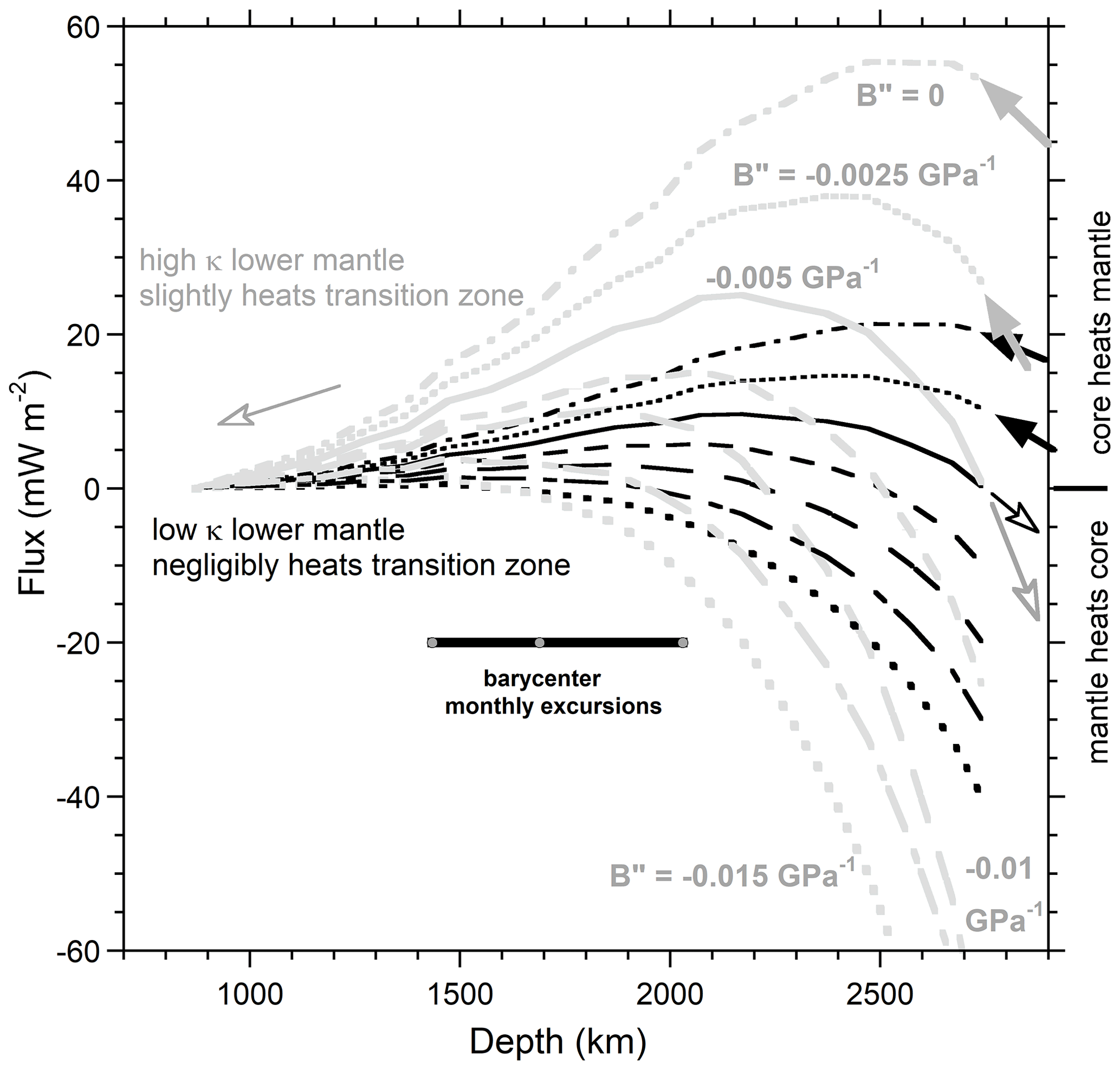
Figure 9Calculated flux for high oxide and low silicate thermal conductivity, as well as various second P derivatives of the bulk modulus, as labeled. The same patterns are used in Figs. 6 and 8. Arrows are extrapolations across D′′, showing that most cases indicate a heat source in the LM. When flux is positive, the temperature is increasing inwards.
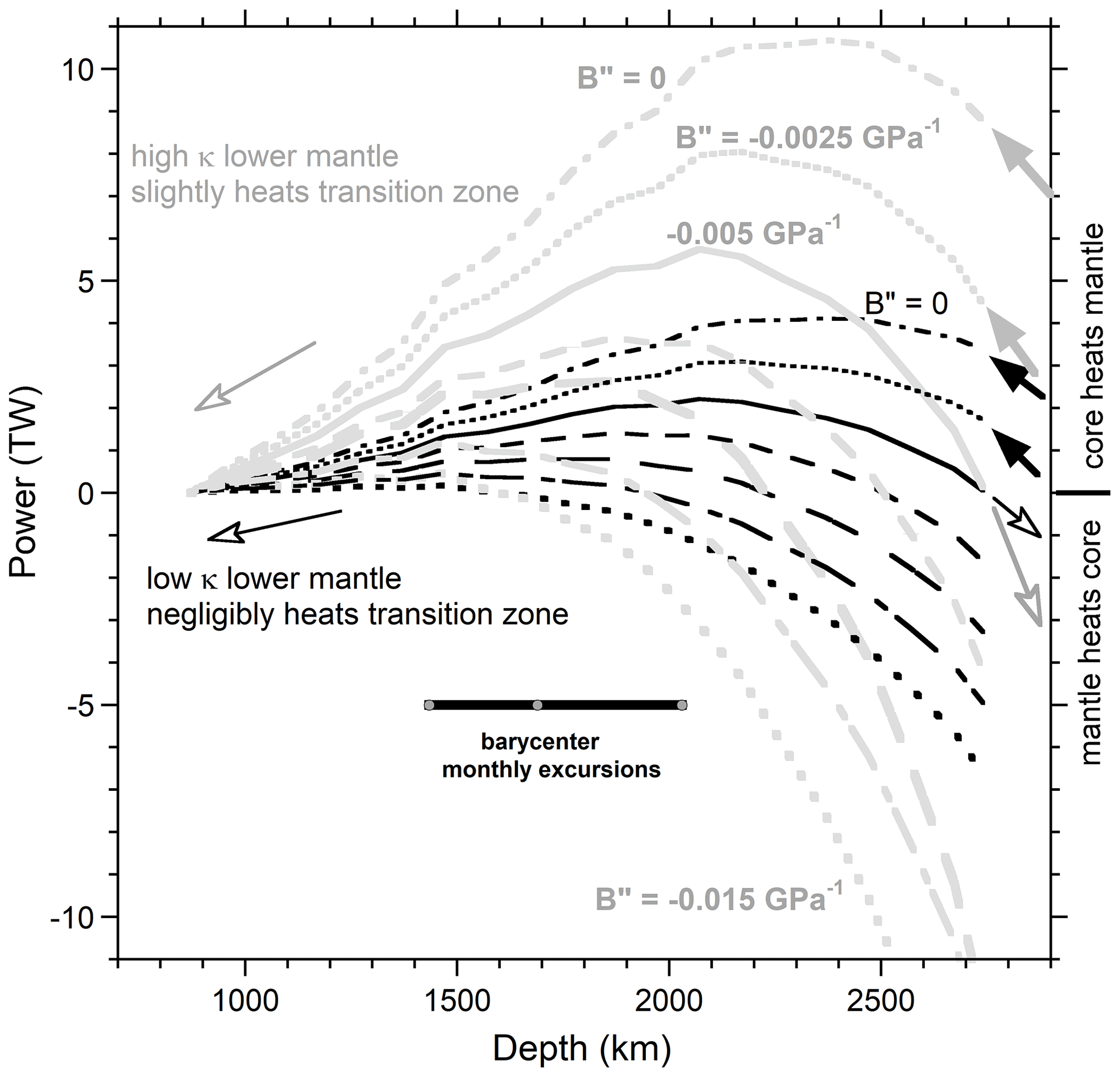
Figure 10Power calculated from the flux curves in Fig. 9 and Eq. (15). Positive power is associated with temperature increasing inwards. Arrows indicate the direction of flow across the core–mantle boundary region and also into the TZ.
Earth's largest zone by mass or volume is the lower mantle, which has only been accessed remotely, via seismic data acquisitions and processing. PREM, Ak135, and other reference models provide nearly identical velocities (Kennett et al., 1995). The models yield smoothly varying properties and their derivatives over most of the LM, the changes of which are taken in this report to represent combined effects of P and T varying with depth. However, a smooth variation in chemical composition is not precluded in utilizing separation of variables (Sect. 2). Gradual changes in chemical composition could be hidden in our choices for B′′ if changes in mineralogy lead to a linear response of . Specifically, mineralogy depending linearly on density and thus on P would lead to an equation equivalent to Eq. (6). Indeed, systematic dependence of velocity (and thus of B) on density exists and has received much attention (see, e.g., the seminal paper of Shankland, 1972). But because varies little among dense phases, as underscored by commonly assuming harmonic values of 4 in analyzing data (see Sect. 2.3), geotherms calculated from PREM via the inverse approach developed here are largely independent of mineralogical details. Values considered for B′′ depict all three different thermal situations that are possible below 670 km: LM temperatures can increase with depth below the TZ, or are constant, or may decrease. Only one case was considered for the last, due to strongly decreasing T being incompatible with a molten outer core (Fig. 8).
The thermal state and gradients inward from the top of the LM indicate that a power source exists in the lower mantle. Locations of the peak in ℘ or flux are little affected by the high-T values of thermal conductivity considered in the inverse model: instead, the location of the power source is largely controlled by B′′. As discussed in Sect. 2.3, B′′ is not well constrained. This ambiguity effectively lumps compositional changes with those solely due to compression. Contrastingly, the heights of the peaks in Figs. 9 and 10 are affected by values for κ and for . Neither variable depends strongly on mineralogy. Note that the large contrast (in κ) explored considers vastly different simple oxide vs. complex silicate compositions.
Notably, thermal models show that the scale length for cooling over geologic time is ∼ 1000 km (Criss and Hofmeister, 2016), so heat generated in the LM cannot reach the surface to any appreciable degree. A similar scale length is obtained from Eq. (2): the Earth cools slowly because it is large and spherical with a refractory outside. Flat geotherms near z = 1000 km with a source near 2000 km are compatible with the thermally insulating nature of rocks and our earlier cooling models. Criss and Hofmeister (2016) used a constant κ that is independent of pressure and so assumed a much more thermally insulating mantle. The flat and low κ case underestimates ℑ in the lower mantle. The consequence is a narrower thermal maxima with little heating of the core in the calculations of Criss and Hofmeister (2016). The broad geotherms inferred from PREM without knowing thermal conductivity are thus consistent with the strong dependence of thermal conductivity on pressure that is demonstrated by experiments (Fig. 2) and, importantly, is inherent to Fourier's definition of ℑ (Sect. 3.3).
In short, results (Figs. 6, and 8 to 10) obtained by analyzing the seismologic representation of Earth's interior are consistent with studies of the equation of state, phase equilibria, and thermal transport properties. Table 1 lists the most likely thermal gradient for the parameters explored. Although other values are possible, the mostly likely gradient is unlikely to change significantly, as likelihood was deduced from melting temperatures for LM and core candidate materials.
Heat is produced in the LM, but how? Commonly considered sources are discussed next. The paper concludes with a proposal.
Heat produced in rocks by radioactive decay has been the focus of many studies. Yet, it is well known that U, Th, and K are concentrated in the continents, leaving very little for the mantle, if meteorites represent the bulk Earth. Flux from the oceans suggests mantle production of <100 W km−3. Such a tiny source can only heat the interior if deeply buried, but for this case excessively high T results, due to the time evolution of the heat-generating isotopes (Criss and Hofmeister, 2016).
This long-standing problem in geochemistry led to considering primordial heat as another source. This hypothesis is based on gravitational contraction producing heat and rests on Kelvin's discounted proposal for the generation of starlight. Changes in gravitational potential produce motions as per elementary physics textbooks. Conversion of gravitational potential to spin and orbits quantitatively accounts for the high kinetic energy for Earth and sister planets today, as well as high spin observed for young stars (see Hofmeister and Criss, 2012). Some accretionary heating is expected in the final stages, but this source is a small fraction of the gravitational potential, non-renewable, shallow, and winding down. Likewise, core formation is not a source of heat: rather, the planet would need to be already melted for a homogeneously accreted object to sort, since self-compression itself provides a stable density stratification.
Heat is a by-product of motions, when accompanied by deformation, non-elastic in particular, or friction. Motions are produced by forces which on large, planetary scales are gravitational in origin. On this basis, and because the previously explored sources of radiogenic and primordial heat are inadequate to describe the workings of Earth (e.g., the hypothesis of mantle convection: see Bercovici, 2007) as well as seismologic detection of a molten core, which is hot, our recent efforts have focused on forces and motions. Hofmeister et al. (2022) argue that the location of the barycenter, where the immense solar pull and orbital centrifugal forces balance, differing from that of the geocenter results in imbalanced stresses and forces that are cyclical with periods of both 1 d and 1 month, with plate tectonics being a consequence. Cyclic stresses promote failure (Schijve, 2009). Spin is important, as the force field is axially symmetric, which explains orientation of the mid-ocean ridge fracture system.
The barycenter is a point in space that the Earth spins through. Its location relative to the geocenter is defined by masses of the Earth and Moon plus the lunar distance, which varies over the month. The depth range of ∼ 1450 to 2050 km, shown in Figs. 8 to 10, includes the position of the power source indicated by B′′ more negative than −0.005 GPa−1. Over the day, this point in space moves through the LM and rarely lies in the equatorial plane, due to Earth's tilted spin axis. Thus, our results for Earth's thermal state are compatible with cyclical stresses heating the LM. This region is strong and plastic (or elastic) rather than brittle, like the lithosphere, but both are underlain by fluid layers. Liquids flow under any stress, the lack of rigidity of which adds stress to the overlying layers. The amount of heat generated is small, ∼ 1 TW, and is conducted away from the source in both directions. Investigating this proposal further is beyond the scope of the present report.
No data sets were used in this article.
The contact author has declared that there are no competing interests.
Publisher’s note: Copernicus Publications remains neutral with regard to jurisdictional claims in published maps and institutional affiliations.
This article is part of the special issue “Probing the Earth: experiments and mineral physics at mantle depths”. It is a result of the 17th International Symposium on Experimental Mineralogy, Petrology and Geochemistry, Potsdam, Germany, 1–3 March 2021.
I thank Robert E. Criss for critical comments.
This research has been partially supported by the National Science Foundation (grant no. EAR-2122296).
This paper was edited by Stephan Klemme and reviewed by two anonymous referees.
Aitta, A.: Iron melting curve with a tricritical point, J. Stat. Mech.-Theory E., 12, P12015, https://doi.org/10.1088/1742-5468/2006/12/P12015, 2006.
Aizawa, Y., Yoneda, A., Katsura, T., Ito, E., Saito, T., and Suzuki, I.: Temperature derivatives of elastic moduli of MgSiO3 perovskite, J. Geophys. Res., 31, L01602, https://doi.org/10.1029/2003GL018762, 2004.
Akaogi, M. and Ito, E.: Heat capacity of MgSiO3 perovskite, Geophys. Res. Lett., 20, 105–108, 1993.
Anderson, D. L.: New Theory of the Earth, 2nd Edn., Cambridge University Press, Cambridge, ISBN 0-86542-335-0, 2007.
Anderson, O. L. and Isaak, D.: Elastic constants of mantle minerals at high temperatures, in: Mineral Physics and Crystallography, A Handbook of Physical Constants, edited by: Ahrens, T. J., American Geophysical Union, Washington D.C., ISBN 0-87590-852-7, 64–97, 1995.
Anderson, O. L., Isaak, D., and Oda, H.: High-temperature elastic constant data on minerals relevant to geophysics, Rev. Geophys., 30, 57–90, 1992.
Andersson, P.: Thermal conductivity under pressure and through phase transitions in solid alkali halides, I. Experimental results for KCl, KBr, KI, RbCl, RbBr and RbI, J. Phys. C Solid State, 18, 3943–3955, 1985.
Andersson, S. and Bäckström, G.: Techniques for determining thermal conductivity and heat capacity under hydrostatic pressure, Rev. Sci. Instrum., 57, 1633–1639, 1986.
Andersson, S. and Dzhavadov, L.: Thermal conductivity and heat capacity of amorphous SiO2: Pressure and volume dependence, J. Phys. Condensed Matter., 4, 6209–6216, 1992.
Bass, J. D.: Elasticity of minerals, glasses, and melts, in: Mineral Physics and Crystallography, A Handbook of Physical Constants, edited by: Ahrens, T. J., American Geophysical Union, Washington D.C., 29–44, ISBN 0-87590-852-7, 1995.
Bercovici, D.: Mantle Dynamics Past, Present and Future: An Introduction and Overview, in: Treatise on Geophysics, Vol. 7, edited by: Schubert, G., 1–30, ISBN 9780444534569, 2007.
Blumm, J., Henderson, J. B., Nilson, O., and Fricke, J.: Laser flash measurement of the phononic thermal diffusivity of glasses in the presence of ballistic radiative transfer, High Temp.-High Pres., 34, 555–560, 1997.
Branlund, J. M. and Hofmeister, A. M.: Thermal diffusivity of quartz to 1000 ∘C: Effects of impurities and the α-β phase transition, Phys. Chem. Miner.., 34, 581–595, 2007.
Cammarano, F., Goesa, S., Vacher, P., and Giardini, D.: Inferring upper-mantle temperatures from seismic velocities, Phys. Earth Planet. In., 138, 197–222, 2003.
Chase Jr., M. W.: NIST-JANAF Thermochemical Tables, Fourth Edition, J. Phys. Chem. Ref. Data Monogr., 9, 1–1951, 1998.
Chopelas, A. and Boehler, R.: Thermal expansivity in the lower mantle, Geophys. Res. Lett., 19, 1983–1986, 1992.
Chudinovskikh, L. and Boehler, R.: Eutectic Melting in the System Fe–S to 44 GPa, Earth Planet. Sc. Lett., 257, 97–103, 2007.
Criss, R. E. and Hofmeister, A. M.: Conductive cooling of spherical bodies with emphasis on the Earth, Terra Nova, 28, 101–109, 2016.
Criss, E. M. and Hofmeister, A. M.: Isolating lattice from electronic contributions in thermal transport measurements of metals and alloys and a new model, Int. J. Modern Phys. B, 31, 75 pp., 2017.
Ditmars, D. A., Ishihara, S., Chang, S. S., Bernstein, G., and West, E. D.: Enthalpy and Heat-Capacity Standard Reference Material: Synthetic Sapphire (α-A1203) from 10 to 2250 K, J. Res. Natl. Bur. Standards, 87, 159–163, 1982.
Dorfman, S. M., Meng, Y., Prakapenka, V. B., and Duffy, T. S.: Effects of Fe-enrichment on the equation of state and stability of (Mg, Fe)SiO3 perovskite, Earth Planet. Sc. Lett., 361, 249–257, 2013.
Dugdale, J. S. and MacDonald, D. K. C.: Lattice thermal conductivity, Phys. Rev., 98, 1751–1752, 1955.
Dziewonski, A. M. and Anderson, D. L.: Preliminary reference Earth model, Phys. Earth Planet. In., 25, 297–356, 1981.
Falloon, T. J., Green, D. H., Danyushevsky, L. V., and McNeill, A. W.: The composition of near-solidus partial melts of fertile peridotite at 1 and 15 GPa: implications for the petrogenesis of MORB, J. Petrol., 49, 591–613, 2008.
Fei, Y.: Thermal Expansion, in: Mineral Physics and Crystallography, A Handbook of Physical Constants, edited by: Ahrens, T. J., American Geophysical Union, Washington D.C., 29–44, ISBN 0-87590-852-7, 1995.
Fiquet, G., Richet, P., and Montagnac, G.: High-temperature thermal expansion of lime, periclase, corundum and spinel, Phys. Chem. Mineral., 27, 103–111, 1997.
Fiquet, G., Auzenda, A. L., Siebert, J., Corgne, A., Bureau, H., Ozawa, H., and Garbarino, G.: Melting of peridotite to 140 Gigapascals, Science, 329, 1516–1518, 2010.
Hahn, O., Hofmann, R., Raether, F., Mehling, H., and Fricke, J.: Transient heat transfer in coated diathermic media: a theoretical study, High Temp.-High Press., 29, 693–701, 1997.
Helffrick, G.: A finite strain approach to thermal expansivity's pressure dependence, Am. Mineral., 102, 1690–1695, 2017.
Hofmeister, A. M.: Interatomic Potentials Calculated from Equations of State: Limitation of Finite Strain to Moderate K′, Geophys. Res. Lett., 20, 635–638, 1993.
Hofmeister, A. M.: Comment on “measurement of thermal diffusivity at high pressure using a transient heating technique” in Appl. Phys. Lett. 91, 181914, 2007, Appl. Phys. Lett., 95, 096101, https://doi.org/10.1063/1.3196374, 2009.
Hofmeister, A. M.: Thermal diffusivity of perovskite-type compounds at elevated temperature, J. Appl. Phys., 107, 103532, https://doi.org/10.1063/1.3371815, 2010a.
Hofmeister, A. M.: Scale aspects of heat transport in the diamond anvil cell, in spectroscopic modeling, and in Earth's mantle, Phys. Earth Planet. In., 180, 138–147, 2010b.
Hofmeister, A. M.: Measurements, Mechanisms, and Models of Heat Transport, Amsterdam, New York, 427 pp., ISBN 978-0-12-809981-0, 2019
Hofmeister, A. M.: Heat Transport and Energetics of the Earth and Rocky Planets, Elsevier, Amsterdam, 350 pp., ISBN 978-0-12-818430-1, 2020.
Hofmeister, A. M.: Dependence of Heat Transport in Solids on Length-scale, Pressure, and Temperature: Implications for Mechanisms and Thermodynamics, Materials, 14, 449, https://doi.org/10.3390/ma14020449, 2021.
Hofmeister, A. M. and Criss, R. E.: A thermodynamic model for formation of the Solar System via 3-dimensional collapse of the dusty nebula, Planet. Space Sci., 62, 111–131, 2012.
Hofmeister, A. M., Dong, J. J., Branlund, J. M.: Thermal diffusivity of electrical insulators at high temperatures: evidence for diffusion of phonon-polaritons at infrared frequencies augmenting phonon heat conduction, J. Appl. Phys., 115, 163517, https://doi.org/10.1063/1.4873295, 2014.
Hofmeister, A. M., Criss, R. E., and Criss, E. M.: Link of planetary energetics to moon size, orbit, and planet spin: a new mechanism for plate tectonics, in: In the Footsteps of Warren B. Hamilton: New Ideas in Earth Science: Geological Society of America Special Paper 553, edited by: Foulger, G. R., Hamilton, L. C., Jurdy, D. M., Stein, C. A., Howard, K. A., and Stein, S., Geological Society of America, Boulder, CO, https://doi.org/10.1130/2021.2553(18), 2022.
Hsieh, W. P., Chen, B., Li, J., Keblinski, P., and Cahill, D. G.: Pressure tuning of the thermal conductivity of the layered muscovite crystal, Phys. Rev. B, 80, 180302, https://doi.org/10.1103/PhysRevB.80.180302, 2009.
Jacobsson, P. and Sundqvist, B.: Thermal conductivity and Lorenz function of zinc under pressure, Int. J. Thermophys., 9, 577–585, 1988.
Kanamori, H., Fujii, N., and Mizutani, H.: Thermal diffusivity of rock-forming minerals, J. Geophys. Res., 73, 595–605, 1968.
Katsura, T.: Thermal diffusivity of silica glass at pressures up to 9 GPa, Phys. Chem. Miner., 20, 201–208, 1993.
Kennett, B. L. N.: On seismological reference models and the perceived nature of heterogeneity, Phys. Earth Planet. Interiors, 159, 129–139, 2006.
Knittle, E.: Static compression measurements of equations of state, in: Mineral Physics and Crystallography: A Handbook of Physical Constants, edited by: Ahrens, T. J., American Geophysical Union, Washington D.C., 98–142, ISBN 0-87590-852-7, 1995.
Konôpková, Z., McWilliams, R. S., Gómez-Pérez, N., and Goncharov, A. F.: Direct measurement of thermal conductivity in solid iron at planetary core conditions, Nature, 534, 99–101, 2016.
Lodders, K. and Fegley Jr., B. J.: The Planetary Scientist's Companion, Oxford University Press, Oxford, ISBN 0-19-511694-1, 1998.
MacDonald, G. J. F.: Calculations on the thermal history of the Earth, J. Geophys. Res., 64, 1967–2000, 1959.
McWilliams, R. S., Konôpková, Z., and Goncharov, A. F.: A flash heating method for measuring thermal conductivity at high pressure and temperature: Application to Pt, Phys. Earth Planet. Int., 174, 24–32, 2015.
Merriman, J. M., Hofmeister, A. M., Whittington, A. G., and Roy, D. J.: Temperature-dependent thermal transport properties of carbonate minerals and rocks, Geophere, 27, 27 pp., https://doi.org/10.1130/GES01581.1, 2018.
Morard, G., Andrault, D., Guignot, N., Siebert, J., and Garbarino, G.: Melting of Fe–Ni–Si and Fe–Ni–S alloys at megabar pressures: implications for the core–mantle boundary temperature, Phys. Chem. Miner., 38, 767–776, 2011.
Mori, Y., Ozawa, H., Hirose, K., Sinmyo, R., Tateno, S., Morard, G., and Ohishi, Y.: Melting experiments on Fe–Fe3S system to 254 GPa, Earth Planet. Sc. Lett., 464, 135–141, 2017.
Murakami, M., Ohishi, Y., Hirao, N., and Hirose, K.: Elasticity of MgO to 130 GPa: Implications for lower mantle mineralogy, Earth Planet. Sc. Lett., 277, 123–129, 2009.
Nestola, F., Burnham, A., Peruzzo, L., Tauro, L., Alvaro, M., Walter, M., and Kohn, S.: Tetragonal Almandine-Pyrope Phase, TAPP: Finally a name for it, the new mineral jeffbenite, Mineral. Mag., 80, 1219–1232, 2016.
Nestola, F., Jung, H., and Taylor, L. A.: Mineral inclusions in diamonds may be synchronous but not syngenetic, Nat. Commun., 8, 14168, https://doi.org/10.1038/ncomms14168, 2017.
Osako, M. and Ito, E.: Thermal diffusivity of MgSiO3 perovskite, Geophys. Res. Lett., 18, 239–242, 1991.
Osako, M., Ito, E., and Yoneda, A.: Simultaneous measurements of thermal conductivity and thermal diffusivity for garnet and olivine under high pressure, Phys. Earth Planet., 143/144, 311–320, 2004.
Pertermann, M. and Hofmeister, A. M.: Thermal diffusivity of olivine-group minerals, Am. Mineral., 91, 1747–1760, 2006.
Ritzwoller, H. and Lavely, E. M.: Three-dimensional seismic models of the Earth's mantle, Rev. Geophys., 33, 1–66, https://doi.org/10.1029/94RG03020, 1995.
Sehlke, A., Hofmeister, A. M., and Whittington, A. G.: Thermal properties of glassy and molten planetary candidate lavas, Planet. Space Sci., 193, 105089, https://doi.org/10.1016/j.pss.2020.105089, 2020.
Shankland, T. J.: Velocity-density systematics: Derivation from Debye theory and the effect of ionic size, J. Geophys. Res., 77, 3750–3758, https://doi.org/10.1029/JB077i020p03750, 1972.
Schijve, J.: Fatigue of Structures and Materials, 2nd Edn. with Cd-Rom, Springer, Berlin/Heidelberg, Germany, ISBN 978-1-4020-6807-2, 2009.
Sinogeikin, S. V. and Bass, J. D.: Single-crystal elasticity of MgO at high pressure, Phys. Rev. B, 59, R14141, https://doi.org/10.1103/PhysRevB.59.R14141, 1999.
Spinner, S.: Elastic moduli of glasses at elevated temperature by a dynamic method, J. Am. Ceram. Soc., 39, 113–118, 10.1111/j.1151-2916.1956.tb15634.x, 2006.
Stachel, T., Harris, J. W., Brey, G. P., and Joswig, W.: Kankan diamonds (Guinea): II. Lower mantle inclusion parageneses, Contrib. Min. Petrol., 140, 16–27, 2000.
Takahashi, E.: Melting of a dry peridotite KLB-1 up to 14 GPa: Implications on the origin of peridotitic upper mantle, J. Geophys. Res., 91, 9367–9382, 1986.
Takeuechi, H., Uyeda, S., and Kanamori, H.: Debate About the Earth. Freeman, Cooper and Co, San Francisco, chap. 6, Is the Earth heating or cooling?, 253 pp., 1967.
Tye, R. P. (Ed.): Thermal Conductivity, Vol. 1–2, Academic Press, London, ISBN 10 0127054014, ISBN 13 9780127054018, 1969.
Vieira, F. and Hamza, V.: Global heat flow: new estimates using digital maps and GIS techniques, Int. J. Terr. Heat Flow Appl. Geotherm., 1, 6–13, 10.31214/ijthfa.v1i1.6, 2018.
Vozár, L. and Hohenauer, W.: Flash method of measuring the thermal diffusivity, A Review, High Temperatures-High Pressures, 35/36, 253–264, https://doi.org/10.1068/htjr119, 2003.
Wallace, D. C.: Thermodynamics of Crystals, John-Wiley and Sons Inc., New York, ISBN 13 978-0486402123, ISBN 10 0486402126, 1972.
Yoneda, A.: Pressure derivatives of elastic constants of single crystal MgO and MgAl2O4, J. Phys. Earth, 38, 19–55, 1990.
Zha, C. S., Mao, H. K., and Hemley, R. S.: Elasticity of MgO and a primary pressure scale to 55 GPa, P. Natl. Acad. Sci. USA, 97, 13494–13499, 2000.
Zhang, J. and Herzberg, C.: Melting experiments on anhydrous peridotite KLB-1 from 5.0 to 22.5 GPa, J. Geophys. Res., 99, 17729–17742, 1994.
Zhao, D., Qian. X., Gu, X., Jajja, S. A., and Yang, R.: Measurement techniques for thermal conductivity and interfacial thermal conductance of bulk and thin film materials, J. Electron. Packag., 138, 040802, https://doi.org/10.1115/1.4034605, 2016.
Zhu, F., Liu, J., Lai, X., Xiao, Y., Prakapenka, V., Bi, W., Alp, E., Przemyslaw, D., Chen, B., and Li, L.: Synthesis, elasticity, and spin state of an intermediate MgSiO3-FeAlO3 bridgmanite: Implications for iron in Earth's lower mantle, J. Geophys. Res.-Sol. Ea., 125, e2020JB019964, https://doi.org/10.1029/2020JB019964, 2020.
- Abstract
- Introduction and background
- Extraction of geothermal gradients from radial seismological models in an inverse approach
- Lower mantle transport properties from theory and experiment
- Results
- Implications and conclusions
- Data availability
- Competing interests
- Disclaimer
- Special issue statement
- Acknowledgements
- Financial support
- Review statement
- References