One-atmosphere high-temperature CO–CO₂–SO₂ gas-mixing furnace: design, operation, and applications

In this paper, we present a new design for a 1 atm gas-mixing furnace using the gas mixture CO–CO₂–SO₂. This furnace can simulate disequilibrium processes such as magmatic and volcanic degassing. Here, we present the technical aspects of the design. The furnace can sustain temperatures of up to 1650 ^∘C and has a hot zone that spans 200 mm vertically, where the hotspot is determined to be ∼ 32 mm below the midpoint of the furnace enclosure. The four mass flow controllers are individually calibrated and accurate to within 0.8 % of the specified value. The fO₂ is accurately reproduced in the furnace within ±0.002 log units, as calibrated by the Fe–FeO reaction across the iron–wüstite (IW) buffer at 1300 ^∘C. The furnace can reliably simulate dynamic conditions, where the fO₂ can be modulated at a maximum rate of 2.0 log units min⁻¹ by varying the gas mixture. A delay of 40 s is observed to attain the fO₂ calculated from the gas mixture, at the hotspot. A series of safety measures to protect the user from exposure to the toxic gases are detailed. In our experiments, the furnace is used to determine sulfur isotope fractionation factors among melt, sulfide, and the gas phase, within a magmatic context, using either crystals of olivine or silica glass tubes. The furnace has the potential to investigate various other dynamic high-temperature reactions occurring on Earth.

1 Introduction

The first person who conducted a petrology experiment using a furnace was Sir James Hall (1806). Since then, numerous high-temperature (HT) petrology studies (Roeder and Emslie, 1970; Lofgren, 1980; Rutherford, 1993; Hammer and Rutherford, 2002) have been conducted to determine the thermodynamic and kinetic parameters of various natural petrologic processes. Today, a vertical HT gas-mixing furnace is an essential instrument in an experimental petrology laboratory. It provides the ability to perform experiments at a high temperature (more than 2200 ^∘C in some cases) within a controlled atmosphere. Several designs (i.e. temperature range, size, gas mixture) are available depending on the application. In general, these apparatuses are designed to maintain a steady temperature and internal atmosphere, at 1 atm, so that chemical and/or isotopic equilibrium can be attained between the condensed phases (liquid or solid) and the surrounding gas. In this contribution, we present a newly designed vertical 1 atm HT furnace, capable of dynamically changing the partial pressure of mixed gas species in the CO–CO₂–SO₂ system during the experiment. Thermodynamic equilibrium between the gas and melt may not be obtained during degassing in the conduit prior to eruption. This is a process that can be simulated with the new furnace configuration (Pichavant et al., 2013; Le Gall and Pichavant, 2016; Moussallam et al., 2022).

The important characteristics of a gas-mixing furnace are the gas mixture, the size of the hotspot, and the quench mechanism. Here, the gas mixture of CO–CO₂–SO₂ is well suited to studying sulfur isotope fractionation among melt, sulfide, and gas. Given the strict safety rules that need to be followed, the design has eliminated any potential exposure to toxic gases and high temperatures. To our knowledge, no studies have reported gas-mixing furnaces that perform systematic changes in the gas mixture during an experimental run. Additionally, few designs use SO₂ in the gas mixture (Haughton et al., 1974; Katsura and Nagashima, 1974; Gaetani and Grove, 1997; Brenan and Caciagli, 2000; O'Neill and Mavrogenes, 2002). Experimental configurations using SO₂ are rare because of the increased toxicity and the potential for S precipitation during cooling to block the extraction pipes. The design by O'Neill and Mavrogenes (2002) is one of the few furnace designs to use a CO–CO₂–SO₂ gas mixture. However, their design cannot be programmed to automatically change the composition of gases during an experiment. Also, their samples are quenched in water, whereas our design uses a cold hollowed-out stainless-steel bolt to quench the sample. While Brenan and Caciagli (2000) used a similar gas-mixing design, the sample was quenched by manually lowering it into an ice–water mixture, a process which is both slow and unsafe. However, the most crucial factors regarding the unique furnace design which is proposed here are the dynamically controlled atmosphere and a large volume. A much larger volume and hotspot allow for larger samples and a variety of sample holders. Increased safety measures also allow for longer experiments with minimal risk of accidental exposure.

2 Design and setup

The description of this 1 atm HT gas-mixing furnace is in three parts: (1) the furnace and sample holder, (2) the gas-mixing unit, and (3) the safety systems.

2.1 Furnace and sample holders

The experimental setup is constructed around a 660 mm tall vertical tube furnace (Elite TSV 17/50/200), with a hot zone rated to be 200 mm vertically and with a maximum temperature of 1700 ^∘C (sustained maximum temperature of 1650 ^∘C). The six heating elements, Kanthal Super 1800, are set in a hexagon around the 60 mm outer diameter (50 mm inner diameter) and 840 mm long alumina tube. Heating is controlled with a Eurotherm 3216CP temperature controller. The top end of the alumina tube is cooled by a water circuit, assuring the electronic components are not exposed to heat and protecting the O-rings which seal the inside of the furnace from the atmosphere.

Our instrument can use one of two ceramic sample holders to set the sample in the hotspot of the furnace. One of them incorporates an oxygen fugacity sensor (ECONOX ContrOx 650) which can be used to calibrate the oxygen fugacity of the system. Both sample holders incorporate a thermocouple (Type B, Pt – 30 % RH vs. Pt – 6 % RH) and a pair of 1 mm thick platinum wires, used as quench electrodes (Fig. 1). The sample holder is introduced from the top of the furnace, and several O-rings prevent gas leaks and seal the inside of the furnace. The sample capsule (olivine crystal or silica tube) is suspended at the end of the sample holder, from the quench electrodes, using a thin platinum wire (diameter: 0.2 mm); this completes the quench current circuit. The sample is quenched by passing an electrical current of 20 A with a maximum DC voltage of 20 V, causing the thin platinum wire to melt, resulting in a drop of the sample to the cold end of the furnace (quench bowl). Typically, fO₂ is calibrated prior to the actual experiment using the sample holder with the oxygen sensor, whereas the simpler sample holder is used for the experiment. This is to safeguard and protect the fO₂ sensor from corrosion (potential reaction with S) during long experiments (6–24 h) as the ceramic sample holder is not perfectly sealed. The calibration also verifies the proper functioning of the mass flow controllers (MFCs) prior to each experiment.

Olivine crystals are used as sample capsules for experiments starting with basalt powder. We use high-Mg olivines (∼ Fo₉₀, purchased from a seller in Arizona who sourced the olivine from peridotites in Pakistan), as they react minimally with basalt and impose a crystal–melt equilibrium which is appropriate for the natural systems investigated. The capsules are machined from whole crystals, rounded, and measure 5–10 mm. Silica glass tubes are used as sample capsules for experiments starting with other materials, such as rhyolite, and metals (Ni, Fe).

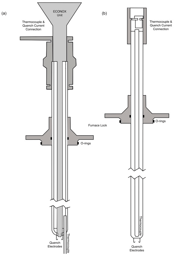
Figure 1 (a) A schematic drawing of the ceramic sample holder with the fO₂ sensor built in. Three connecters at the top: one for the fO₂ sensor to the ECONOX ContrOx 650 controller; the other from the thermocouple to the computer; and the last one the reference air inlet, which is pumped in with a pump built into the ECONOX controller. At the lower end: two 1 mm thick platinum wires with hooks (quench electrodes) and the thermocouple which extends out to roughly the height at which the sample is suspended. This sample holder has a total length of 68 cm. (b) A schematic drawing of the simple ceramic sample holder. At the top: the connector which transmits the current from the thermocouple to the computer. At the lower end: two 1 mm thick platinum wires with hooks (quench electrodes) from which the sample is suspended. This sample holder has a total length of 62 cm.

2.2 Gas-mixing unit/control interface LabVIEW

The gas-mixing unit was designed to ensure the safety of the operator; therefore, the gas flow is controlled by a computer placed in a separate room. Furthermore, the four gas tanks (Ar, CO, CO₂, SO₂) are stored in a cabinet with an exhaust vent, next to the furnace. Four Alicat mass flow controllers for Ar (model MC, range up to 1000 cm³ min⁻¹), CO (model MC, range up to 500 cm³ min⁻¹), CO₂ (model MC, range up to 1500 cm³ min⁻¹), and SO₂ (model MCS, range up to 400 cm³ min⁻¹) are also placed inside the cabinet. Only a single gas line with the mixed gas leaves the cabinet and is connected to the alumina tube of the furnace. The mass flow controllers are chosen to achieve 3.4 mm s⁻¹ flow velocity (400 cm³ min⁻¹) in the alumina tube, and Ar is used to flush the system at a rate of 8.5 mm s⁻¹ (1000 cm³ min⁻¹). The mass flow controllers are controlled through a LabVIEW control interface, developed specifically for this furnace (Fig. 2), which enables dynamic control of the MFCs during an experiment and records temperature and gas flow rates. In brief, the control signal is sent to a mass flow controller from the independent unit (National Instruments cRIO-9066) which communicates with the control interface in the PC. This unit is also designed to control the security actions in case of component failures, such as overheating, malfunction of the air extraction system, and detection of toxic gases above safety thresholds. Gas set-point files are loaded into the control interface as .csv files and are used to control the gas flow rates during an experiment.

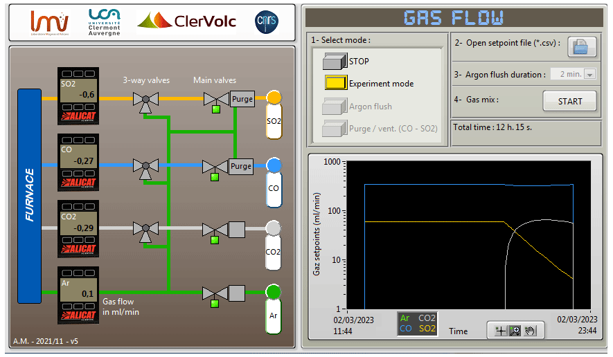
Figure 2 A screenshot of the LabVIEW interface that controls the gas-mixing part of the furnace. The panel on the left visualizes the gas cabinet schematics to show the valve status (open green and closed grey) and display the values from the gas mass flow controllers. The panel on the right is used to set and control the gas flow values. This figure shows the associated change in the gas mixture for a dynamic change in fO₂ and fS₂ after 8 h of equilibrium. It also provides options for argon flush and purging the CO and SO₂ lines.

2.3 Safety systems

The safety of the user against exposure to toxic gases and high temperatures was a priority in this design; therefore multiple safety features were set in place.

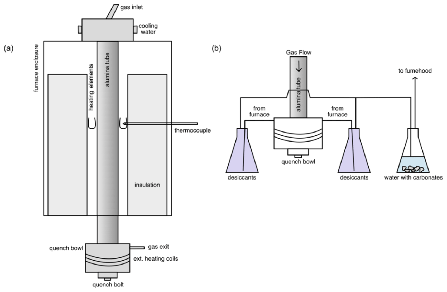
Figure 3 (a) A schematic diagram of the furnace showing the ceramic insulation, U-shaped MoSi₂ heating elements, thermocouple, and alumina tube within the furnace body. At the top is the gas entry and at the bottom the quench bowl and the gas exit. (b) A schematic diagram of the downstream assembly. The stainless-steel quench bowl is heated to ∼ 160 ^∘C with the external heating coil to prevent the build-up of sulfur. The gas leaves through two exits, each going into a beaker containing desiccants to precipitate sulfur. The gas is then collected from the bottom of the beaker and sent into the third beaker containing water with carbonates to react with CO₂ and SO₂. Via another tube, the gas is then let into the fume hood which releases the gas into the atmosphere at the roof.

The CO and SO₂ lines are connected to a security box that keeps the gas valves closed until the safety relay is activated. This system is connected to the gas sensors and the fume hood sensor in the room; if they exceed safety thresholds or if the fume hood stops functioning, the valves are automatically shut. The gas is cleaned downstream by passing it through two glass beakers with desiccants to get rid of moisture (that might come from the third beaker) and to precipitate sulfur. The dry gas then goes on to a third glass beaker and is bubbled in water with some carbonates to dissolve CO₂, whereas the SO₂ reacts with carbonates to form sulfates. A minimal amount of CO is also dissolved. The remaining gas is then fed straight into the evacuation hood, all while keeping the entire system closed (Fig. 3). The furnace room is also evacuated by an additional fume hood to ensure maximum safety in case of a leak elsewhere. The fume hoods evacuate the room at a rate of 125 L s⁻¹. Using a Dräger X-am 2500 portable gas detector at the roof exit, it was determined that of the gas used, roughly 98 % of the CO and 1 % of the SO₂ are released into the atmosphere. Therefore, the CO concentration is within the 8 h exposure limit (<50 ppm) at the roof exhaust. Additionally, the CO and SO₂ have extra gas lines for purging to ensure a safe release of the tank when they need to be replaced.

The safety of the operator is assured by a portable gas sensor which is typically placed near the furnace, in addition to the array of fixed gas detectors. Human presence in the furnace room is minimized. An Internet protocol (IP) camera is used to monitor the system remotely. In case of a leak, masks designed to filter out SO₂ and CO are available. In case the cooling water stops flowing for any reason, the safety mechanism automatically stops the furnace to prevent overheating.

3 Operation

The furnace is usually kept at 700 ^∘C and is heated to the experimental temperature as the first step. The fO₂ sensor bearing sample holder is then introduced and lowered to the hotspot, and the furnace is flushed with Ar for approximately 5 min, which corresponds to a volume several times the size of the system. The desired gas mixture is passed through for ∼ 30 min until a stable fO₂ reading is recorded. Once again, the system is flushed with Ar. The fO₂ sensor bearing sample holder is then swapped out for the simple holder that suspends the prepared sample. At this point, the sample is placed near the top of the furnace, which is ∼ 600 ^∘C cooler than the hotspot. The furnace is immediately flushed with argon to prevent the occurrence of any reaction with air. The sample is gradually lowered to the hotspot in about four to five steps over 30 min; this is done to avoid thermal shock to the sample capsule, as some olivine crystals have invisible micro-defects that might result in them breaking apart due to the thermal shock. Once the thermocouple reads a temperature that is 20–25 ^∘C from the target, the experiment is started with the flow of the CO–CO₂–SO₂ gas mixture. The flow of the gas mixture immediately raises the temperature by approximately 5 ^∘C, likely due to the change in the thermal conductivity. The bubbling of the outgoing gas is monitored in the third beaker with water. The bubbling is typically intermittent and is considered a reliable indicator of normalcy. The intermittence is likely caused by the CO₂ dissolution into the water, and there are no such observations for the Ar gas flow. The gas mass flow controllers are also closely monitored for the first 30 min of the experiment to ensure stability. At the end of the experiment, the sample is quenched into the hollowed quench bolt (a piece in the centre, Fig. 4) in the bottom bowl of the furnace. The quench bowl is heated to a temperature of ∼ 160 ^∘C during the experiment with a heating coil to prevent sulfur precipitation. This temperature was chosen as it is sufficiently hotter than the melting point of S (112.8 ^∘C) and lower than the melting point of the O-rings. The quench bolt is cooled externally with a beaker of cold water prior to dry-quenching the sample, which falls into the cooled inner quench bolt. The inner bolt is clean, dry, and free of sulfur, as any sulfur liquid drips down pools outside the outer S-drain bolt. The gas flow and the heating coil are then stopped; the furnace is flushed with argon for 5 min before recovering the sample. The furnace is then cooled down to its idle temperature of 700 ^∘C.

Figure 4 A schematic diagram of the quench bowl. The sample falls into the inner “quench” bolt, while the “S-drain” bolt traps sulfur that is dripping down from the sides of the alumina tube. Prior to the quench, the head of the bolts are cooled externally. This dry-quench setup facilitates better control over S precipitation and allows for longer-duration experiments.

4 Calibration and performance

4.1 Temperature calibration

4.1.1 Thermocouple calibration

The accuracy of the thermocouple (Type B) on the simple ceramic sample holder was determined by melting a pure gold metal strip. The strip was suspended across the platinum quench electrodes of the sample holder, and the height of the holder was adjusted so that the strip was at the hotspot. The temperature was then raised to 1100 ^∘C on the temperature controller, and the system was left to equilibrate until the temperature measured by the thermocouple remained constant. The set temperature on the controller was then increased by 1 ^∘C every 2 min until the Au strip melted. The resistance across the quench electrodes was measured using a voltmeter (∼ 1.5 Ω) to determine when the Au strip melted. A minute after the set temperature on the controller reached 1110 ^∘C, the resistance jumped to 0.5 MΩ, indicating that the circuit was open due to the gold melting. At that moment, the temperature indicated by the thermocouple, adjusted for its distance from the hotspot, was 1061.3 ^∘C, which soon stabilized to 1062 ^∘C. Accounting for hysteresis, the melting temperature of Au is 1064.43 ^∘C (Haynes et al., 2016); therefore, the thermocouple records temperatures 2.43 ^∘C colder than the actual temperature.

4.1.2 Hotspot position

Determination of the hotspot location was carried out at temperatures of 1200, 1300, and 1400 ^∘C, which were set using the temperature controller, with a steady flow of Ar at 3.4 mm s⁻¹ (400 cm³ min⁻¹), representative of the experimental gas flow rate and temperature. Results show that the hotspot is located at ∼ 32 ± 2 mm (Fig. 5), below the midpoint of the furnace enclosure. The location of the hotspot at each temperature is nearly the same, and the shift is insignificant. The hotspot location is also found to be independent of the gas flow rates for the range of 1.7–6.8 mm s⁻¹ (200–800 cm³ min⁻¹). An offset of 46–52 ^∘C is observed in the temperature range of 1200–1400 ^∘C between the two thermocouples, due to their position. The thermocouple used by the temperature controller is outside the alumina tube, whereas the recorded temperature is from the thermocouple on the ceramic sample holder within the furnace and records a lower temperature. No change in this offset has been noted in over 200 experiments. The temperature variation at the hotspot is within 10 ^∘C over 5 cm, giving the gas mixture approximately 7 s to react completely at the desired temperature before reaching the hotspot and the sample.

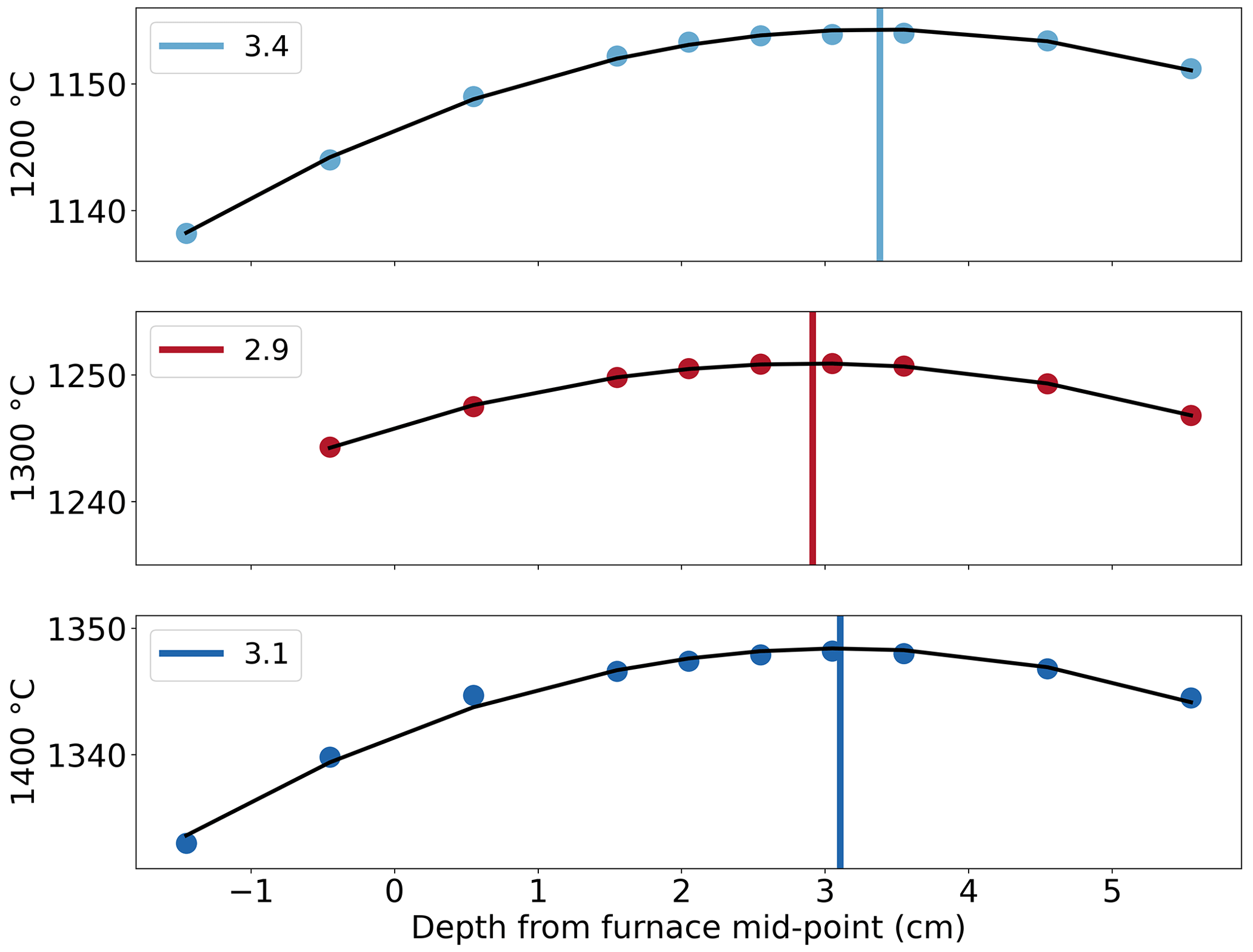
Figure 5 Temperature measured vs. depth from the midpoint of the furnace. y-axis labels indicate the temperature set at the controller, which reads a higher temperature near the heating element. The curve was derived from a square fit and then maximized to find the location of the hotspot.

4.2 Mass flow controller performance

The performance of the mass flow controllers (MFCs) was inspected from the log produced by the control interface. They are precise and send the requested flow of gas with an error of ±2 cm³ min⁻¹. According to Alicat, the MFCs for CO, CO₂, and Ar have a precision of ±0.6 % of the reading or ±0.1 % of the full scale (±0.8 % of the reading or ±0.2 % of the full scale for SO₂), whichever is greater. It is attempted to keep the values for individual gases above 20 cm³ min⁻¹ (0.17 mm s⁻¹), at which errors are 5 % relative to the requested flow rate. This lower limit of the MFC sets the lower limit of attainable fS₂ in the furnace, indicated by the field in Fig. 8. The use of an MFC capable of regulating lower flow rates can allow further reduction of fS₂ in the gas mixture.

4.3 fO₂–fS₂ calibrations

The atmosphere in the furnace is controlled by the thermodynamic equilibrium imposed by the mixture of the gases and the temperature. Here, the partial pressures of nine gas species are calculated (O₂, CO, CO₂, COS, CS₂, S₂, SO, SO₂, SO₃) by Gibbs-free-energy minimization using iterative Lagrangian optimization (modified from an open-source code, Thermochemical Equilibrium Abundances (TEA), developed by Blecic et al., 2016, based on the methods of Eriksson et al., 1971, and White et al., 1958, using thermodynamic data from Chase, 1998). Based on the Gibbs-free-energy minimization mentioned above, Fig. 6 shows the range of fO₂–fS₂ conditions that can be attained in the furnace at 1300 ^∘C, using the gas mixture CO–CO₂–SO₂. The gas mixture begins to react as it enters the top of the furnace. When it reaches the 200 mm long hotspot (50 mm long within 10 ^∘C), the mixture is expected to be fully reacted and consists of the equilibrium gas species as calculated above.

The fO₂–fS₂ condition within the furnace was calibrated in steps. First, fO₂ control was verified using the Fe–FeO and Ni–NiO reactions at their respective buffers ( iron–wüstite (IW) and NNO) followed by tests using the fO₂ sensor. Once calibrated for fO₂, fS₂ was calibrated by the synthesis of FeS or magnetite at the FeS–magnetite buffer.

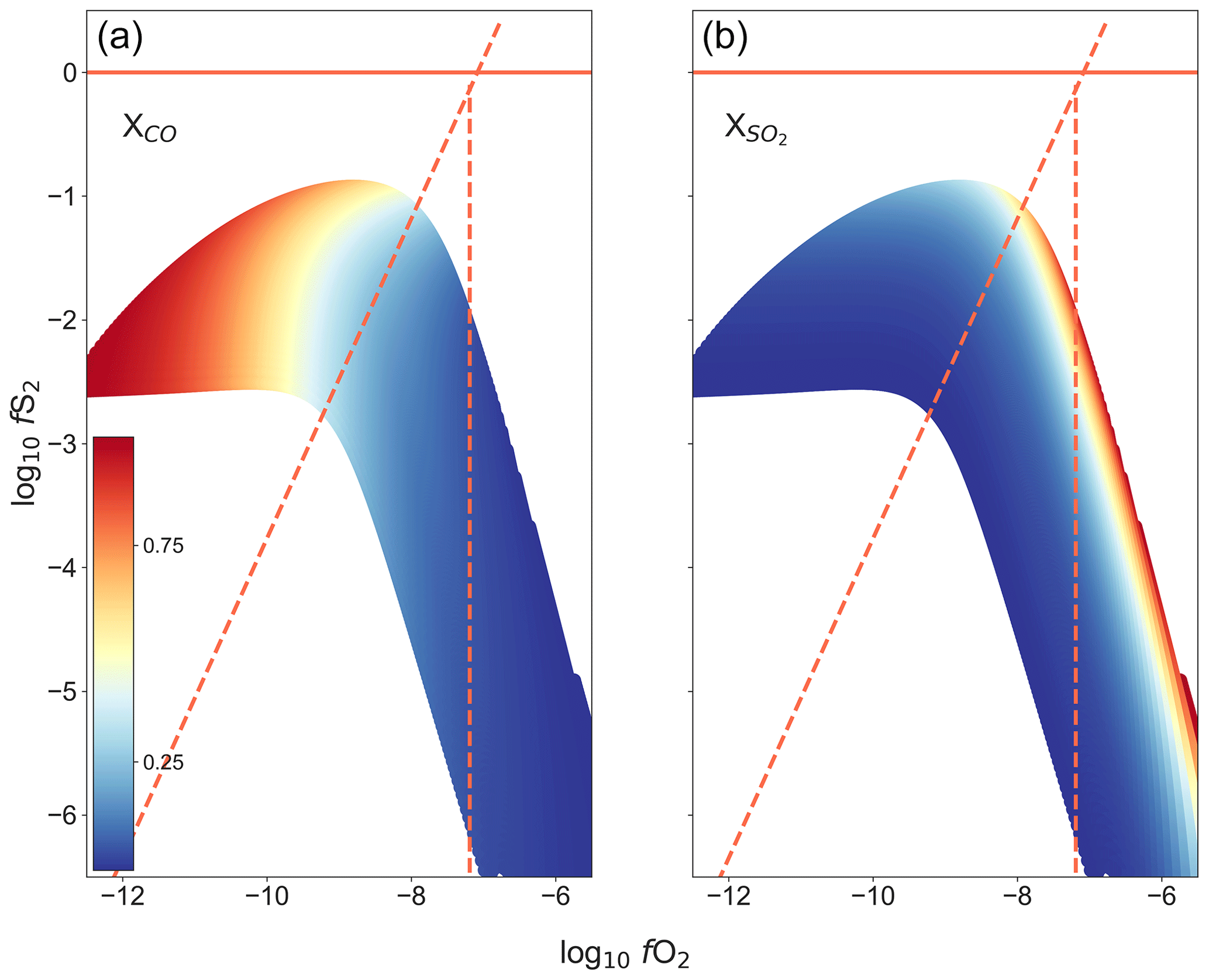
Figure 6 The range of fO₂–fS₂ conditions that can be attained within the furnace at 1300 ^∘C, using the gas mixture CO₂–CO–SO₂. Calculated using Gibbs-free-energy minimization. Panel (a) shows the proportion of CO in the gas mixture, while (b) shows the proportion of SO₂ in the gas mixture. The redlines show the limits of the reaction boundaries as reference, sloped line: 3FeS + 2O₂ = Fe₃O₄ + $\mathrm{3}/\mathrm{2}$ S₂, vertical line: 3Fe₂SiO₄ + O₂ = 2Fe₃O₄ + 3SiO₂.

The fO₂ condition within the furnace can be monitored using a Y-doped zirconia sensor and mineral reactions. The mineral reactions used were the Fe–FeO and the Ni–NiO reactions. Both were tested using different methods. The fO₂ condition was verified at the NNO buffer by an oxidation reaction of Ni metal (Ni–NiO, Ni + $\mathrm{1}/\mathrm{2}$ O₂ NiO), which was visually determined after quench. Two experiments (Table 2), starting with pure NiO powder, in a Si glass capsule were carried out at 1350 ^∘C. In both cases, the result follows expectations; i.e. we have NiO at a positive NNO condition and Ni at a negative NNO condition. Based on the above calibration, the fO₂ condition within the furnace is accurate to within ±0.27 log fO₂.

The fO₂ condition was verified at the IW buffer (Fe–FeO, Fe + $\mathrm{1}/\mathrm{2}$ O₂ FeO) at 1300 ^∘C by measuring the resistance across a 1 mm wide pure Fe strip suspended between the Pt quench electrodes. The log fO₂ was varied from −11.5 to −10 in 30 min. The log fO₂ according to the gas mixtures calculated at 1300 ^∘C was varied from −11.5 to −10 in 30 min. The equilibrated T at the hotspot was 1288.3 ^∘C. In these conditions, IW = 0 at log fO₂ = −10.8826. The initial resistance across the Fe strip was 2.53 Ω. The resistance stayed constant for ∼ 5 min and then slowly started increasing at the rate of 0.02–0.04 Ω min⁻¹. A minute after crossing the buffer (calculated from the gas flow values at the MFCs), the resistance starts increasing dramatically (>0.2 Ω min⁻¹), and within 5 min, the strip breaks (likely due to fast conversion to FeO). Given a 40 s travel time for the gas from the MFC to the hotspot, the corrected log fO₂ at the time of crossing the buffer is −10.886. Based on this assessment criteria, the fO₂ is accurate to within ±0.002 log fO₂.

The zirconia sensor works by measuring the potential difference generated by the difference in oxygen activity at both ends (gas mixture and reference air). The fO₂ at the sample location is calculated using the following formula (derived from Nernst's law):

$$\log p{\mathrm{O}}_{\mathrm{2}}=-{\displaystyle \frac{\mathrm{mV}}{\left(\mathrm{0.0496}\cdot T\right)}}+\log p{{\mathrm{O}}_{\mathrm{2}}}_{\mathrm{ref}},$$

where mV is the potential difference detected by the sensor in millivolts, T is the temperature in kelvin, pO${}_{{\mathrm{2}}_{\mathrm{ref}}}$ is the reference pressure of oxygen in bars (0.21 is used), and pO₂ is the partial pressure of oxygen at the location of the sensor in bars. The constant value of 0.0496 is derived from the equation $\frac{\mathrm{2.303}\cdot R}{n\cdot F}$, where R is the gas constant; F is the Faraday constant; 2.303 is the conversion factor from natural log to log₁₀; and n equals 4, since four electrons are exchanged in the reaction between the zirconia membrane, the reference air (atmosphere), and the atmosphere of the furnace. The location of the zirconia sensor is 3 cm above the sample; however the temperature of the thermocouple of the sample holder is applied to the equation to determine the fO₂ at the sample location. We tested attainment of target fO₂ conditions by running experiments under several gas mixtures for 30 min each at temperatures of 1200–1400 ^∘C (Table 1). We observed that the atmosphere within the furnace appears to be more oxidizing (by about 0.4 log units) than expected from the gas mixture (i.e. the sensor reads higher fO₂). The shift observed is independent of the gas proportions introduced and flow rate. We conclude this is a shift in the zero point of the sensor and that the absolute readings of the sensor are not a reliable representation of the atmosphere within the furnace. However, the zirconia sensor accurately tracks the changes in the fO₂ conditions of the furnace. This is discussed further in the following section (Sect. 4.4). We therefore conclude that the fO₂ sensor in our possession is inaccurate but precise.

Table 1 fO₂ calibration runs.

^a The expected fO₂ condition, as calculated from the gas mixture. ^b The measured fO₂ condition using the fO₂ sensor.

With the fO₂ calibrated, reversal experiments were run to calibrate fS₂ and ensure the target condition is accurately attained. Since an fS₂ sensor does not exist, calibrated redox conditions were used to verify the sulfide's formation and disappearance. These experiments follow the standard operating procedure outlined in Sect. 3. Here, the key reactions taking place in this system are as follows:

$$\begin{array}{}\text{(R1)}& {\displaystyle }\mathrm{2}\mathrm{CO}\left(\mathrm{g}\right)+{\mathrm{SO}}_{\mathrm{2}}\left(\mathrm{g}\right)\rightleftharpoons \mathrm{2}{\mathrm{CO}}_{\mathrm{2}}\left(\mathrm{g}\right)+\mathrm{1}/\mathrm{2}{\mathrm{S}}_{\mathrm{2}}\left(\mathrm{g}\right),\text{(R2)}& {\displaystyle }\mathrm{2}{\mathrm{CO}}_{\mathrm{2}}\left(\mathrm{g}\right)\rightleftharpoons \mathrm{2}\mathrm{CO}\left(\mathrm{g}\right)+{\mathrm{O}}_{\mathrm{2}}\left(\mathrm{g}\right),\text{(R3)}& {\displaystyle }\mathrm{3}\mathrm{FeS}\left(\mathrm{s}\right)+\mathrm{2}{\mathrm{O}}_{\mathrm{2}}\left(\mathrm{g}\right)\rightleftharpoons {\mathrm{Fe}}_{\mathrm{3}}{\mathrm{O}}_{\mathrm{4}}\left(\mathrm{s}\right)+\mathrm{3}/\mathrm{2}{\mathrm{S}}_{\mathrm{2}}\left(\mathrm{g}\right).\end{array}$$

Reaction (R3) describes the exchange of sulfide or oxide, and as fO₂ is calibrated and controlled by the gas mixture, fS₂ can be determined once the equilibrium boundary of the reaction is experimentally determined. Practically, the reaction boundary needs to be bracketed using Reaction (R3) by starting with FeS and Fe₃O₄.

The precise details of these experiments are provided in Table 2. Figure 7a shows the sample (no. 179) that started out with pure Fe powder and is now an iron sulfide. For this starting condition, the iron metal is expected to quickly react to form metastable oxide (3Fe+2O₂Fe₃O₄) and sulfide (2Fe+S₂2FeS) before transforming into the equilibrium phase. Figure 7b is a BSE image of the sample (no. 163) that started out with pure FeS₂ powder and was oxidized to form an iron oxide, most likely Fe₃O₄. For this starting condition, the disequilibrium FeS₂ reacts to form iron oxide. Since this experiment was run for just 2 h and at a lower temperature, some cores (brighter part) of unreacted iron sulfide are visible in the image (Fig. 7b). Based on these observations, we conclude that the fS₂ imposed by the gas mixture reflects that of the calculation. Figure 8 indicates the conditions of all sulfide-forming experiments and one iron oxide formation (no. 163). The horizontal axis is fO₂ relative to the fayalite–magnetite–quartz buffer (Frost, 1991), and the vertical axis is fS₂ relative to Reaction (R3). All our experiments are consistent with the expected boundary of Reaction (R3), and the boundary is bracketed within ±0.6 log units of fS₂. However, given the accuracy of the MFCs in reproducing the fO₂ values accurately, we see no reason why the fS₂ values should be significantly off. We can therefore safely assume that the fS₂ accuracy of the furnace is as good as the fO₂ accuracy.

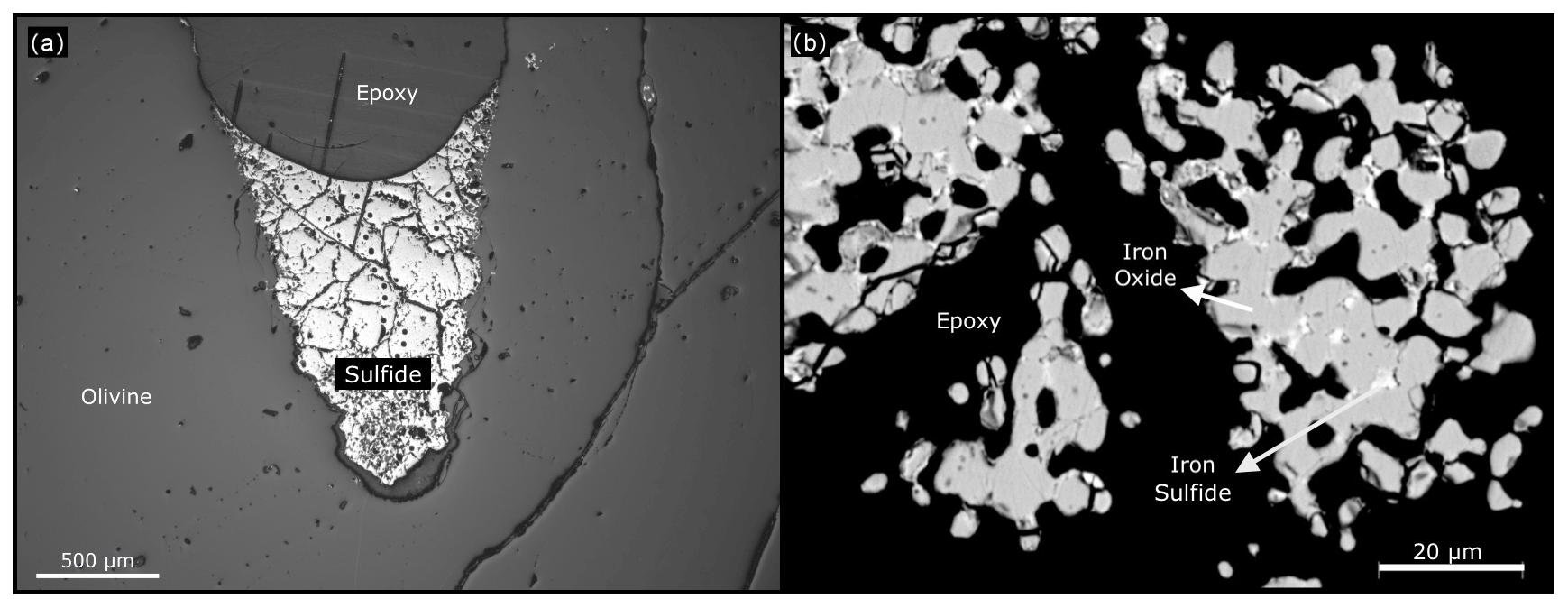
Figure 7 (a) At the end of the 8 h experiment at 1300 ^∘C with fS₂ within sulfide stability, the gold-coloured material, iron sulfide, is formed. Image from a petrological microscope. (b) In this BSE image, we can still observe cores of iron sulfide in some of the grains. Running the experiment for longer periods of time and at higher temperatures would oxidize them.

Table 2 fO₂–fS₂ calibration experiments.

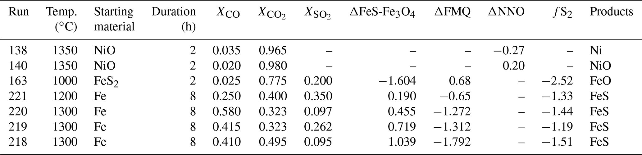
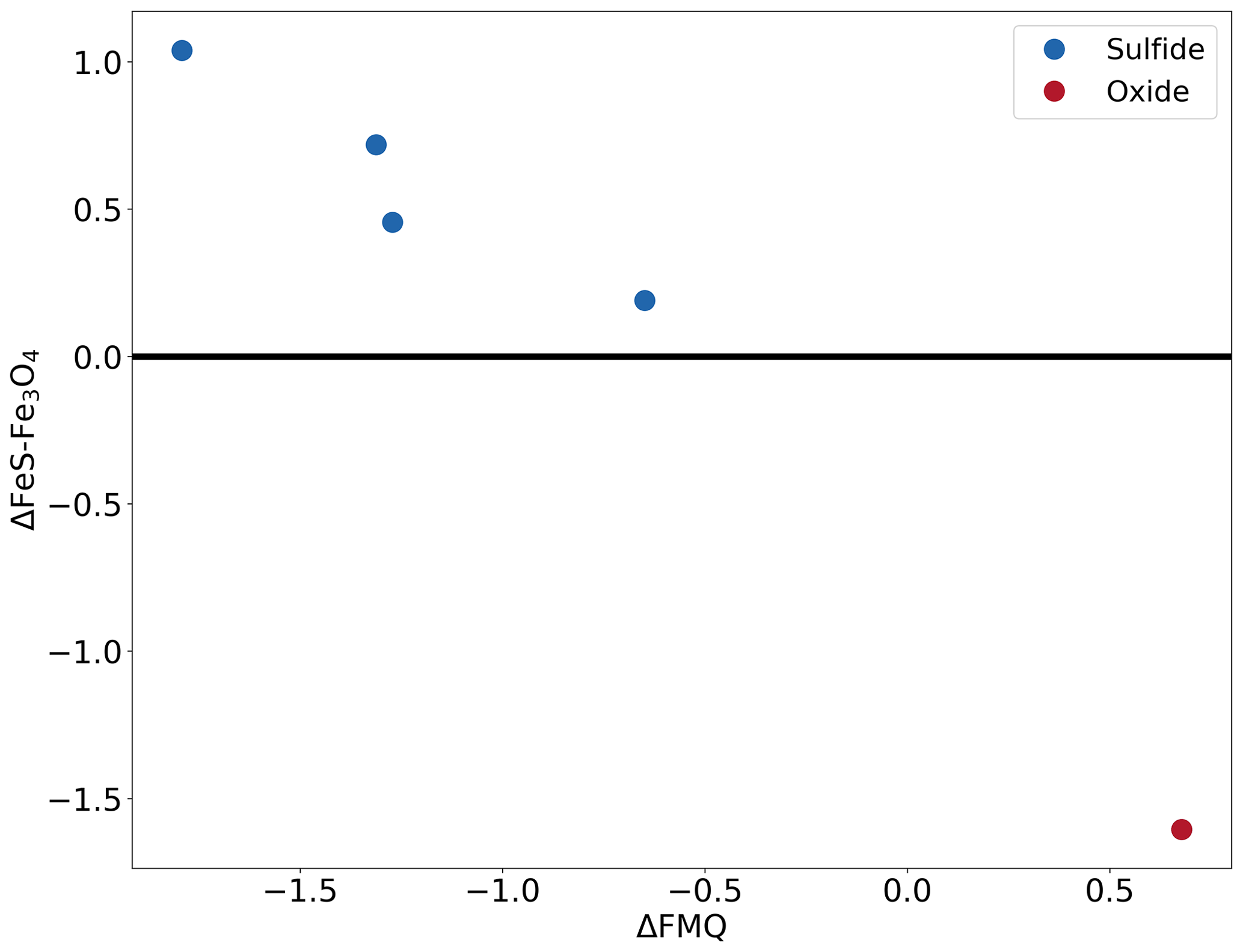
Figure 8 The conditions of the different experiments that formed sulfide and oxide. The x axis shows the fO₂ condition relative to the quartz–fayalite–magnetite buffer. The y axis shows the fS₂ condition relative to the reaction 3FeS + 2O₂ ⇌ Fe₃O₄ + $\mathrm{3}/\mathrm{2}$ S₂. This figure is temperature independent as the x and y axes are referenced relative to the buffers, allowing for the depiction of all the experiments in one figure.

4.4 Dynamic conditions

To perform experiments that simulate conditions of degassing, it is necessary to constrain which fO₂ conditions in the furnace can be dynamically controlled and the rates at which they can be changed. There exists an upper limit to how fast the atmosphere within the furnace can be changed, as fast changes in the gas mixture may be dampened during transport. The limit was determined by continually modifying the gas mixture in the furnace at fixed time intervals by creating steps in the gas set-point file. A constant flow rate of 400 cm³ min⁻¹ was used during this calibration. Figure 9 shows the result of the calibration, in which the fO₂ was varied sinusoidally between −7.3 and −11.2 with a period of 12 min, thereby changing fO₂ at an average rate of 1.294 log units min⁻¹, with a maximum of 2.032 log units min⁻¹. It was observed that the fO₂ values track linearly with the changes in the gas with a delay of 40 s. This corresponds to the transport time from the MFCs to the hotspot. Therefore, the setup reliably simulates this pace of fO₂ change. The tests with shorter periods at 2, 4, and 8 min reproduced the sinusoidal curves, but the amplitude of these curves was dampened, indicating diffusion and/or incomplete reaction within the gas mixture during transport (not shown here).

Figure 9 Changes in fO₂ in the furnace plotted against time (s). Red dots show the fO₂ values calculated from the gas flow rates. The gas mixture was changed at a maximum rate of 2.032 log units min⁻¹. The condition inside the furnace is monitored by an oxygen fugacity sensor (blue circles). Tested with CO–CO₂ gas mixture.

The typical “degassing” experiment imposes a constant rate of change in fO₂ and fS₂ after the system reaches equilibrium. Such experiments simulate certain degassing conditions observed in nature, such as the ones modelled by Burgisser and Scaillet (2007). This constant change in the fO₂ and fS₂ of the system requires precise management of the gas flow rates as they are not linear or systematic. The degassing path is divided into multiple sub-steps, and the corresponding gas mixture is calculated for each point and interpolated between them. The points are closely spaced where the changes in the gas mixture are greatest. Based on the previous oscillation experiment, the duration of the change can be reduced to approximately 5 min, and it is possible to simulate a 1 log unit change in partial pressure of oxygen and sulfur. Based on a coupled chemical–physical model calculation, fS₂ in a magma can change by approximately 0.6 log units as it ascends from 1 kbar to the surface (Burgisser and Scaillet, 2007).

5 Potential applications

The creation of a gas-mixing furnace that can faithfully replicate equilibrium and disequilibrium conditions lends itself to plenty of potential applications in high-temperature, near-surface geology, especially volcanology. In addition to the direct applications discussed in the Introduction, other potential applications are discussed below:

1. High-temperature and lower-pressure conditions are believed to cause significant sulfur isotope fractionation between gas species, melt, and sulfides (de Moor et al., 2013; Mandeville et al., 2009; Marini et al., 2011, 1998; Sakai et al., 1982); such fractionation can be replicated and quantified.

2. Quantifying the behaviour of sulfur and the amount of oxygen in the sulfide, the Fe and Ni content in the associated melt in various oxygen and sulfur fugacity conditions is of great interest (Brenan and Caciagli, 2000; Mungall et al., 2005; Shima and Naldrett, 1975) and can tell us more about the accumulation of chalcophile elements in sulfide and their associated melts (Holzheid and Lodders, 2001; Parat et al., 2011; Rose and Brenan, 2001). This is of great importance as many chalcophile elements are economically important and understanding the behaviour of sulfur and its isotopes in volcanic and magmatic processes can improve our understanding of how and where deposits of these chalcophile elements might have formed or may form in the future (Kiseeva et al., 2017; Kiseeva and Wood, 2015).

3. Volcanic degassing processes are known to cause isotopic and elemental fractionation in a wide range of elements (Mandeville et al., 2009; Sossi et al., 2019; Vlastelic et al., 2021). This fractionation occurs in dynamic conditions where temperature and gas compositions change with time. Many questions also exist around the HT reactions that take place at volcanic craters, fumaroles, and vents (Kusakabe et al., 2000; Shinohara et al., 2015; Vlastelic et al., 2021). By determining the isotopic fractionation factors between gas, melt, and sulfide in equilibrium and disequilibrium conditions, we can estimate critical parameters related to degassing processes, such as the ascent rate of the magma or residence time of the magma in the reservoir. The known isotopic composition of the gas used in the experiment can be used to characterize the gas–melt fractionation. This is because the input gas floods the system and, given the minute size of the sample, the overall isotopic equilibrium of the system is controlled by the gas composition. To experiment with disequilibrium conditions, multiple experiments are carried out, and each is stopped at a different point to capture compositional and isotopic snapshots of the melt. The melt exchanges sulfur isotopes with a gas with a constant isotopic composition but varying molecular species, which imposes disequilibrium.