the Creative Commons Attribution 4.0 License.
the Creative Commons Attribution 4.0 License.
 | 28 Sep 2022
The hierarchical internal structure of labradorite
Hans-Joachim Kleebe
Ute Kolb
The different structural features of labradorite and its incommensurate atomic structure have long been in the eye of science. In this transmission electron microscopy (TEM) study, all of the structural properties of labradorite could be investigated on a single crystal with an anorthite–albite–orthoclase composition of An53.4Ab41.5Or5.1. The various properties of labradorite could thus be visualized and connected to form a hierarchical structure. Both albite and pericline twins occur in the labradorite. The size of alternating Ca-rich and Ca-poor lamellae could be measured and linked to the composition and the color of labradorescence. Furthermore, a modulation vector of 0.0580(15)a* + 0.0453(33)b* − 0.1888(28)c* with a period of 3.23 nm was determined. The results indicate an eα labradorite structure, which was achieved by forming Ca-rich and Ca-poor lamellae. The average structure and subsequently the incommensurate crystal structure were solved with a three-dimensional electron diffraction (3DED) data set acquired with automated diffraction tomography (ADT) from a single lamella. The results are in good agreement with the structure solved by X-ray diffraction and demonstrate that 3DED–ADT is suitable for solving even incommensurate structures.
- Article
(14109 KB) - Full-text XML
-
Supplement
(1013 KB) - BibTeX
- EndNote


1.1 General information
Labradorite is part of the plagioclase series, which ranges between the endmembers albite (Ab; NaAlSi3O8) and anorthite (An; CaAl2Si2O8), with labradorite existing in the composition range between An50 and An70 (Okrusch and Matthes, 2013). The cell parameters in this compositional range of labradorite vary between a = 8.1668–8.1809 Å, b = 12.8509–12.8723 Å, c = 14.2086–14.2148 Å, α = 93.5802–93.5325∘, β = 116.23–116.1817∘, γ = 89.8396–90.387∘ and Z = 8 with a cell volume of 1334.53–1339.8 Å3 (Jin and Xu, 2017a; Jin et al., 2020). It reveals cleavage planes along (001) (perfect) and (010) (good) and is frequently twinned according to the albite or pericline laws. Polysynthetic twins are often seen on (001) or (010) (Okrusch and Matthes, 2013). In addition to twinning, labradorite contains a variety of different structural features, including a 3–6 nm modulated superstructure exhibiting e- and f-satellites (Fig. 1), a 20–50 nm domain texture, and, in addition, a lamellar structure that is ∼ 100 nm in size and causes the well-known schiller, also called labradorescence (Olsen, 1977). Labradorescence describes an interference with light on lamellae that are all oriented in the same direction, which causes a play of color that can range over the entire spectrum of the visible light (Bøggild, 1924). Labradorite may contain many inclusions, which are typically irregularly distributed within the crystal, with the most common ones being iron oxides such as hematite, magnetite or ilmenite (Henn et al., 2020). However, they do not affect the occurrence of labradorescence (Raman and Jayaraman, 1950).
1.2 Labradorescence
In bright-field transmission electron microscopy (BF-TEM) images, the lamellae of labradorite are alternating light and dark regions (Bolton et al., 1966). Depending on composition, their size can vary between 50–250 nm (Miúra, 1978). They are in principle periodic but tend to branch out leading to a lack of long-range order. The phase boundaries between the lamellae are coherent (Smith and Brown, 1988). The lamellae merge without defects or structure stresses because there is only a slight difference in cell parameters in the plagioclase series of 0.1 %, and the γ angle differs by only 0.4 % (Hoshi et al., 1996). This has been observed by a minor splitting of Kikuchi lines (Nissen, 1971; Nissen et al., 1973; Hoshi et al., 1996).
Labradorescence occurs because of optical interference of the lamellar structure (Bolton et al., 1966; Smith, 1974). The wavelength of the intensity maximum of the reflecting light, i.e., the color of the iridescence, can be explained by Bragg diffraction on a stack of varying thickness (Bolton et al., 1966). Lamellae can form along several orientations, but most often, the labradorescence is seen in the direction of the b axis. That is, most lamellae are approximately parallel to the (010) plane (Bolton et al., 1966; Smith and Brown, 1988; Hoshi et al., 1996). Several sources claim the labradorizing plane deviates from the (010) plane by approximately 14–15∘ (Lord Rayleigh, 1923; Raman and Jayaraman, 1950). The labradorescence may be interrupted by non-labradorizing parts; at such boundaries, the labradorite then always shows dark blue colors (Bøggild, 1924) due to the lamellae becoming smaller until reaching a size that only reflects UV light in the non-labradorizing areas. The lamellae differ in Ca and Na content (Nissen et al., 1973), with the broader lamellae being Ca-rich, while the narrower lamellae are enriched in Na (Hoshi et al., 1996). The composition of the Ca-poor and Ca-rich lamellae differs by up to 12 %. In addition, all labradorites with schiller have an orthoclase (Or) content greater than 2 mol% (Nissen et al., 1973). With increasing An content, the size of Ca-rich lamellae increases rapidly, and the size of Ca-poor lamellae decreases slowly in proportion (Smith and Brown, 1988). The thicker the lamellae are, the higher the wavelength λ of the scattered rays is, ranging from dark blue to red. Based on the work of Bolton et al. (1966) an equation was established by Miúra et al. (1975) that displays the origin of the respective color of labradorite. Additionally, regression equations for the wavelength λ and thus the An content, depending on the lamellar thickness d, were derived:
For a more detailed discussion of the derivation of the equations given above, please see Sect. S1 in the Supplement.
1.3 Spinodal decomposition
It is likely that the labradorite lamellae are formed by spinodal decomposition. Distinguishing spinodal segregation from nucleation is possible only in the very early stages of maturation (Smith and Brown, 1988). At low temperatures and slow diffusion rates, there is a possibility that even over long periods of time the process will not progress beyond the spinodal stage. The chemical fluctuations are periodic and can be described as sinusoidal modulations in composition. Their wavelength is usually between 50 and 500 Å. Labradorite shows typical indications of a spinodal decomposition process in TEM such as a periodic modulation with diffuse boundaries, in which the diffraction pattern of a single phase shows satellite reflections (Putnis, 2001).
1.4 e-plagioclase
Most compositions in the plagioclase series crystallize in a structure, the high-albite structure. In An-rich compositions, the structure changes to the body-centered space group due to an increasing Al : Si ratio. In the compositional range in between albite and anorthite, neither of these ordering schemes are possible. The deviations from the 1 : 3 and 1 : 1 Al : Si ratios of the endmembers lead to an unfavorable energetic situation (Putnis, 2001). By reorganizing the structure and ordering the atomic positions, the energy of the solid solutions can be minimized. Since the Al–Si distribution is coupled to the Na–Ca distribution, and the Al–Si ordering schemes are fundamentally different in albite and anorthite, this results in an incommensurate structure with satellite reflections of different periodicity imposed on the main reciprocal lattice (Kitamura and Morimoto, 1977). The superstructure is composed of a modulation wave that describes the displacement and density change in all atoms in the average structure. In general, Na atoms remain in the central part of their position in the structure, while Ca atoms lie further away from their center. Thus, the larger the electron density offset is, the more Ca-rich the composition is. The modulation was assigned to arise from the Ca and Na positions (Xu et al., 2016), which also has a great influence on the distribution of Al and Si atoms in the tetrahedra (Kitamura and Morimoto, 1977). This represents a compromise for the ordering; however, it satisfies local charge balances. Thus, the structures e1 and e2 are formed, which are Ca-rich and Na-rich, respectively (Putnis, 2001). Therefore, various miscibility gaps exist in the plagioclase series. At ∼ An50, a discontinuity occurs in the spacing and orientation of the satellites, as well as the cell parameters and solution enthalpy. This way e1 and e2 are easily distinguished from each other (Putnis, 2001). This marks the position of the Bøggild miscibility gap in which lamellar intergrowths of e1 and e2 are formed. Various endmember compositions of the Bøggild intergrowth are given in the literature with An40–An50 (Hoshi et al., 1996; Putnis, 2001), An35–40–An50–55 (Nissen, 1971), An44–45 (lower limit) (Jin and Xu, 2017a), An47–An53 (Smith and Brown, 1988), An51–An50 (Bøggild, 1924) and An45–An65 (Okrusch and Matthes, 2013).
In intermediate plagioclases An25–75, only major reflections (a-reflections) with occur (Fig. 1). All plagioclases with more than An55 show the f-reflections around the a-reflections. These are second-order satellite reflections that are very faint but intensify with high anorthite content (Smith and Brown, 1988). Xu et al. (2016) discovered the f-reflections in a Na-rich (An49) e-plagioclase for the first time. In addition, a pair of extra satellite reflections (e-reflections) with a center of mass at a*, b*, were observed, indicating absent b-reflections and thus a doubling of the c axis (Fig. 1). The e-reflections were first described by Chao and Taylor (1940) and later by Hoshi et al. (1996), Kalning et al. (1997), Nakajima et al. (1977), and Xu et al. (2016).
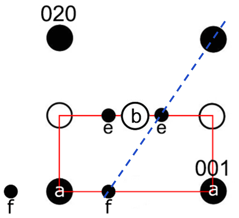
Figure 1Schematic drawing of a reflection arrangement along the zone axis [100]. The labradorite cell, which is displayed in red, is simplified (90∘ angle and distances not to absolute scale). The f-reflections occur around the a-reflections, while the e-reflections occur around absent b-reflections. The satellites are connected with the a-reflections in a straight line (dashed blue line).
The existence of satellite reflections results from a modulation of the ordering scheme. Their position and hence the direction of the modulation is described by the vector t that consists of δh, δk and δl (∈R), with its origin being at the absent b-reflections (Kitamura and Morimoto, 1977). The direction of the modulation runs perpendicular to t, with a thickness of t. The thickness and direction change with increasing An content (Xu et al., 2016). Thereby, the wavelength of the modulation also increases with increasing An content (Smith and Brown, 1988). The satellite reflections change continuously in orientation and spacing over the course of the lamellae (Hoshi et al., 1996; Nissen et al., 1973). For plagioclase, the t vector has a magnitude of about 3–6 nm (Kalning et al., 1997).
The e-plagioclase structure has long been considered metastable because Al–Si diffusion seemed too slow for equilibrium to be reached. However, some reasons support their actual stability. First, natural potassium feldspars can also reach a high Al–Si degree of order at temperatures of a few hundreds of degrees Celsius. Moreover, Al–Si diffusion distances of at least 100–200 nm are possible in the plagioclase structure, as shown by the occurrence of lamellae of this order in labradorite (Carpenter, 1986). Additionally, the modulation period does not get longer as the cooling rate of e-plagioclase decreases: it gets longer with increasing An content (Jin and Xu, 2017b).
2.1 Sample preparation
For transmission electron microscopy (TEM) studies powdered samples and ion-milled samples were prepared. In the case of the powdered samples, a small piece of labradorite was mortared and suspended in ethanol before being dripped onto a carbon-coated copper grid. For the ion-milled samples, a piece of labradorite was ground using a tripod MultiPrep™ from Allied High Tech Products, Inc., Rancho Dominguez, CA, USA, until the thickness was below 30 µm. After gluing the samples onto molybdenum grids, they were ion-milled with a DuoMill 600 from Gatan, Pleasanton, CA, USA. A 15∘ angle was used for the Ar ion beam. Initially, a voltage of 4 kV was used, which was reduced to 3.5 kV as thinning progressed. The ion beam was always kept between 0.75–1 mA per gun. Finally, the samples were thinned again at 1 kV for 15–20 min to gently remove the amorphized surface. To avoid electrostatic charging of the samples under the incident electron beam, they were lightly coated with carbon.
2.2 Light microscopy
A polarizing microscope (Zeiss Axio Lab.A1, Carl Zeiss AG, Oberkochen, Germany) was used for the initial examination of the samples and to depict initial characteristics.
2.3 Transmission electron microscopy (TEM)
All TEM investigations were performed with a JEOL 2100F, Tokyo, Japan (200 kV), or a FEI Tecnai F30, Eindhoven, Netherlands (300 kV). A 2k × 2k charge-coupled device (CCD) camera (Ultrascan100 from Gatan, Pleasanton, CA, USA) was used at the JEOL. A tomography attachment for the JEOL single tilt holder was used as a sample holder. Energy dispersive X-ray spectrometry (EDS) was performed using an X-Max80 detector from Oxford Instruments, High Wycombe, UK. A 4k × 4k CCD camera (Ultrascan4000 from Gatan) and a tomography sample holder from E. A. Fischione Instruments Inc., Export, PA, USA, were used with the FEI instrument. EDS was performed with an EDAX detector (Mahwah, NJ, USA). For scanning transmission electron microscopy (STEM), a high angular annular dark-field (HAADF) detector was used. For automated diffraction tomography (ADT) measurements, a Fast-ADT measurement routine was utilized as a plug-in for DigitalMicrograph 3, for TEM mode (JEOL) and for STEM mode (FEI) (Plana-Ruiz et al., 2020). ADT was performed in nano-beam diffraction mode (NBD), which allows the beam to be kept quasi-parallel up to 20 nm. In this way, crystallites in the nanometer range can also be processed, which is not possible with X-ray diffraction (Kolb et al., 2012). Since the beam can be reduced in size down to the nanometer range in this mode, diffraction images with a good signal-to-noise ratio can be acquired even from single nanoparticles (Zuo and Spence, 2017). Electron beam precession (PED) was performed by the NanoMEGAS (Brussels, Belgium) DigiStar program.
2.4 Automated diffraction tomography
Automated diffraction tomography (ADT) was used to record the three-dimensional diffraction data of a crystal. It is best performed on small, thin single crystals in a range of about 100 nm in size. ADT was performed in nano-beam diffraction mode. In the case of JEOL 2100F, the smallest spot size of 0.5 nm was used. Which α is selected depends on the beam size. To be able to obtain three-dimensional diffraction data, a tilting series of diffraction patterns was recorded. To ensure that the crystal does not move off axis during tilting, the eucentric height was mechanically adjusted first. Because the crystal still moved back and forth during the tilting process, even if the eucentric height was set correctly, a tracking file was recorded, which served as a reference image. In the images of the tracking file the region of interest (ROI) was marked. The beam was set to a size of 50–200 nm. The value of the condenser lens 2 (CL), was saved to facilitate a return to this beam size. Then the beam shift was calibrated using the X and Y deflections of the beam. The beam was then set to the ROI and changed to diffraction mode. The diffraction image was centered, and the exposure time was adjusted so that the camera was not overexposed. Finally, the initial parameters were loaded, and the Fast-ADT routine was started (Plana-Ruiz et al., 2020).
When using ADT with fixed tilt steps, the reciprocal space is sampled more finely, and therefore more diffraction points can be captured compared to diffraction images limited to zone axes. In terms of tomography, the two-dimensional diffraction images are then merged to form a three-dimensional space. Orienting the crystal before taking the sequence is not necessary and should even be avoided to capture more independent reflections. In addition, the diffraction images of zone axes have particularly many dynamic effects. Thus, non-oriented crystallites contain fewer dynamical effects and provide pseudo-kinematic data sets. Since the use of the NBD mode results in small disks from the diffraction points, the diffraction image must be refocused via the intermediate lens because otherwise the disks could overlap, in particular, for large unit cells. This changes the effective camera length, which must be calibrated. The precession of the electron beam during the ADT measurement captures more diffraction points between the tilt steps and generates fewer dynamic effects because intensities are integrated instead of just intersected, a precession angle of 0.5–1∘ being sufficient (Kolb et al., 2012).
The obtained three-dimensional reciprocal space was then analyzed with the programs eADT (Kolb et al., 2012) and PETS (Palatinus et al., 2019). Here the cell parameters and space group can be determined. The cell parameter determination has an accuracy of 1 %–2 %. The cell has to be multiplied by a factor to calibrate the effective camera length, allowing for the extraction of the intensities from the raw data. This data set was then used for the structure solution in SIR2019 (Burla et al., 2015) and Jana2006 (Petříček et al., 2014). The crystal structures were visualized with VESTA 3 (Momma and Izumi, 2011).
In the past scientific work was published dealing with the solution of incommensurate structures with three-dimensional electron diffraction (3DED). Palatinus et al. (2011) used the charge flipping algorithm to solve the hexagonal incommensurate structure of η′- from 3DED data. Other works by Boullay at al. (2013), Lanza et al. (2019), and Plana-Ruiz (2020) show the application of 3DED to solve orthorhombic materials modulated along a main axis, and Steciuk et al. (2016) published a paper on solving a monoclinic, layered ferroelectric material, with a modulation vector showing components of two axes.
3.1 Sample preparation
The labradorite used for the electron microscopic examinations was from Toliara Province, Madagascar (Fig. 2b). The crystal exhibits labradorescence from dark blue to yellow and is strongly twinned (Fig. 2a). To ensure consistency, all samples were taken from an area of yellow labradorescence. In addition to powdered samples, ion-milled samples were also prepared. In order to reach all major axes and thus allow a comprehensive characterization, three sections at 90∘ to each other were prepared, with one being cut parallel to the labradorescence. Perpendicular to this, two sections were cut at 90∘ with one perpendicular to the labradorescence and the macroscopic twins. The other cut section was also perpendicular to the labradorescence but running parallel to the observed twins.

Figure 2(a) Sample of labradorite displaying labradorescence ranging from dark blue to yellow. The samples were taken in a yellow area (lower left corner). Additionally, polysynthetic twinning can be seen. (b) Map of Madagascar with Toliara Province, the place of discovery of the labradorite, marked in yellow (ESRI, 2011). The sample shown in (a) is from the southern area of Ampanihy, Atsimo-Andrefana, marked in red.
3.2 Transmission electron microscopy (TEM)
Since the labradorite sample turned out to be electron beam sensitive, the TEM examinations were performed with a medium spot size of around 4 nm and the second largest condenser aperture with a diameter of 100 µm. If the electron beam remained on one spot for a longer period of time, radiation damage could still be detected. In this case, an even smaller spot size or condenser aperture was selected for imaging. ADT was performed with the smallest condenser aperture (10 µm), which reduced the electron dose even more and thus prevented sample damage during measurement.
A total of 15 ADT data sets were taken from all three ion-milled samples. The best data set was recorded with Fast-ADT in STEM mode in a tilt range of −60 to +60∘ with a beam size of 150 nm, a camera length of 1 m, an exposure time of 1 s per frame and a precession angle of 1∘. The satellite reflections were clearly visible in the electron diffraction images obtained.
Some structures of labradorite can already be seen by the naked eye or at relatively low magnifications under an optical microscope; however, for the purposes of this research and in order to image all structural aspects, mainly electron microscopy was employed for investigating the internal hierarchical structure of labradorite.
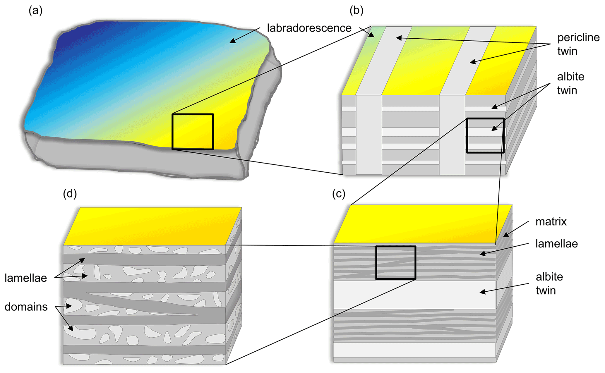
Figure 3Not-to-scale schematic drawing of the different structures in labradorite. (a) Macroscopically, the labradorescence, ranging from dark blue to yellow, can be seen. Panel (b) represents a magnified view from (a). Here, the albite (0.2–1 µm) and pericline twins (∼ 200 µm) are shown. (c) Magnifying the area around the albite twins even further reveals the presence of alternating thicker and thinner lamellae (∼ 100 nm) that are approximately parallel to each other and lie in the plane of labradorescence. (d) An even higher magnification additionally showing small domains (20–50 nm) being present only in the bigger lamellae.
In the following, the different structural features shown in Fig. 3, starting with the albite and pericline twins, will be presented and separately discussed.
4.1 Twins
Two different types of polysynthetic twins were found in this labradorite: albite and pericline twins (Fig. 4a). Pericline twinning can already be seen with the naked eye (Fig. 2), while albite twinning only becomes visible under crossed nicols in a polarizing microscope (Fig. 4b). When viewed approximately along the a axis, both twins can be observed in a single cut. Albite twins are typically 0.2–1 µm wide. At an angle of about 90∘, these are intersected by much larger pericline twins about 200 µm in size. Albite twins are not present in the pericline twins. In the TEM, diffraction images of the zone [100] taken at the twin boundary of an albite twin show split diffraction spots along the c* axis, resulting in and (Fig. 5a). When a dark-field image is produced from a diffraction spot along the or axis, the diffraction contrast originates only from either the matrix or the twin, respectively (Fig. 5b and c). Accordingly, the diffraction image of a pericline twin boundary shows a split b* axis, creating and (Fig. 5d). As with the albite twinning, the dark-field images of diffraction spots along the or axis also show only the matrix or the twin illuminated (Fig. 5e and f). Thus, the diffraction pattern containing the or axis arises from the matrix, while the pattern containing the or axis is produced by the respective twins.
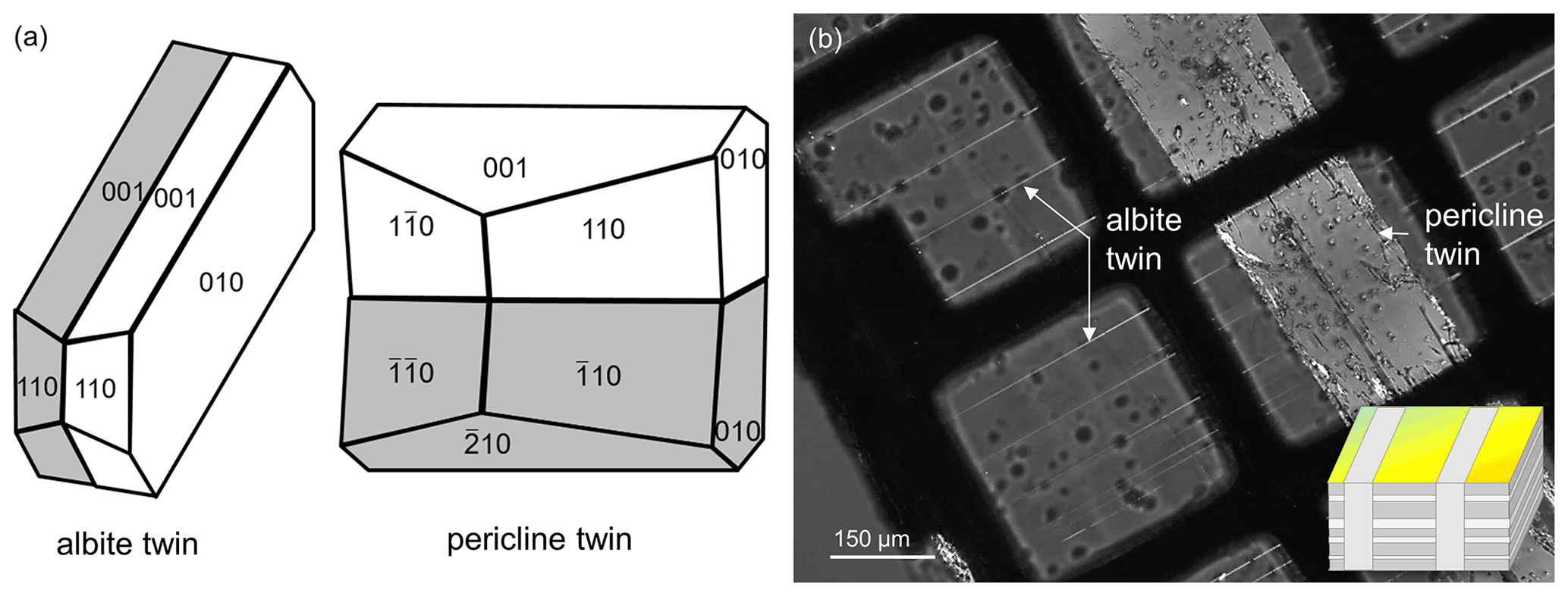
Figure 4(a) Schematic drawing of an albite and a pericline twin in labradorite. (b) Labradorite that was cut at 90∘ to the twinning and the labradorescence under crossed nicols in a polarizing microscope. Besides the pericline twins, there are polysynthetic albite twins that are intersected by the pericline twins at an angle of about 90∘. Note that no albite twins were observed inside the pericline twin. Insert in the bottom-right corner of (b) was taken from Fig. 3.
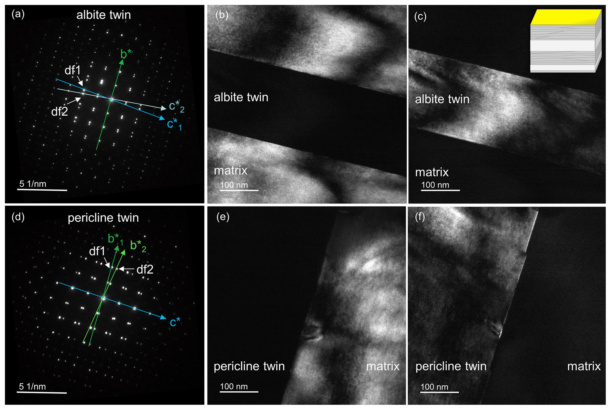
Figure 5TEM images of twinning in labradorite. Panels (a)–(c) show the twin boundary of an albite twin, while (d)–(f) show the twin boundary of a pericline twin. (a) Diffraction pattern along the zone axis [100]. The splitting of the diffraction spots can be seen along c*, resulting in and . (b) Dark-field image of df1, which lies in the direction . The diffraction information arises from the matrix, while in (c), the dark-field image of df2 (lying on ), only the albite twin is illuminated. (d) Diffraction pattern along the zone axis [100]. The diffraction spots are split along the b* axis, creating and . (e) Dark-field image of df1, which lies on the direction . Only the matrix is illuminated, while in (f), the dark-field image of df2, which lies on , only the diffraction information from the pericline twin is shown. Insert in the top-right corner of (c) was taken from Fig. 3.
4.2 Lamellae and local domains
In the samples that were cut perpendicular to the labradorescence plane, alternating thick and thin lamellae were seen in bright-field (BF) imaging. Apart from a few intersections, the lamellae run mostly parallel to each other. In the pericline twins, the lamellae are oriented differently and meet the lamellae from the matrix at an acute angle.
In the TEM, the lamellae can be better visualized in dark-field (DF) mode. Depending on which diffraction spots are used for dark-field imaging (Fig. 6a), different features of the labradorite become visible. In order to make the lamellae visible, 020 was selected for dark-field imaging because it shows a strong difference in diffraction contrast for the Ca-rich (dark) and Ca-poor (bright) lamellae (Fig. 6b). The boundaries of the lamellae are diffuse since there is not an instant but only a gradual change in composition from one lamella to the next.
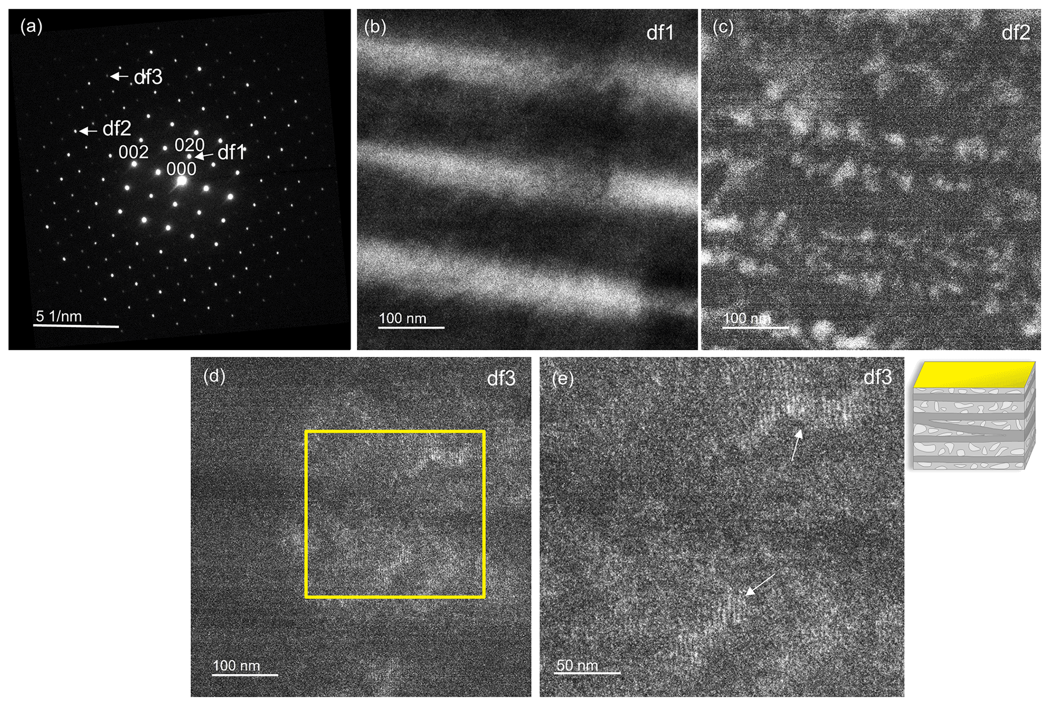
Figure 6(a) TEM diffraction image along the [100] zone axis of the labradorite matrix. Selected diffraction points df1–df3 are marked by arrows and displayed in TEM dark-field images (b–e). (b) Dark-field image of 020 where the Ca-rich (dark) and Ca-poor (light) lamellae are visible. (c) Dark-field image of a pair of e-satellites between 014 and 015. Domains in the lamellae become visible. (d) Dark-field image of 064. The yellow framed area is enlarged in (e) and displays e-fringes in some areas with a distance of approximately 3 nm. Insert to the right of (e) was taken from Fig. 3.
In the TEM image shown in Fig. 6c, utilizing a pair of e-satellites for dark-field imaging, additional ∼ 50 nm domains with diffuse boundaries are visible only in the Ca-rich lamellae; however, none were found in the Ca-poor lamellae. These could have been formed during the phase transition from the high-temperature phase to the low-temperature e-plagioclase, similar to experimental results of Benna et al. (1995) and Németh et al. (2007) with Sr-feldspar and Ca-rich plagioclase, respectively. In the domains, approximately 3 nm large e-fringes can be seen (Fig. 6d and e), which arise from the modulation and run perpendicular to the vector t.
The lamellae are not fully perpendicular to the b axis. In fact, they are tilted ∼ 11∘ away from it. In order to determine the thickness of the lamellae, 232 of the thick and 232 of the thin lamellae each were measured. The thicker lamellae have an average thickness of 129 nm, while the thinner lamellae are about 64 nm thick. Only lamellae that were parallel to each other were taken into consideration.
In order to determine the differences in the composition of the various lamellae, an energy dispersive X-ray spectroscopy (EDS) line scan was performed over seven lamellae (Fig. 7) in STEM mode. The number of counts of the elements was first related to the total counts for each distance to correct for thickness. Then it was multiplied by the k factor of each element. The weight percentage (wt %) thus obtained was converted to mole percentage (mol%). The average composition determined of the yellow regions was Ca0.53Na0.42K0.05Si2.43Al1.53Fe0.04O8. Evaluation of the EDS line scan shows that the thicker, lighter lamellae were more enriched in Ca and depleted in Na, while the opposite was true in the thinner, darker lamellae. The trend of the content of Al, Si, K and Fe is displayed in Fig. 8. As expected, in the Ca-rich lamellae the Al content also increases, while the Si content decreases (Fig. 8a). Considering the general formula for plagioclase Ca1−xNaxAl2−xSi2+xO8, with x ranging from 0 to 1, the determined variation in the Si and Al content can be explained. For the Fe content, although the noise in the EDS spectra is rather high due to the low count rate for Fe, a slight trend can be discerned in Fig. 8b, which follows that of the Al content across the lamellae. This may result from the fact that Fe can be incorporated in the tetrahedral position replacing Al3+ (Makada et al., 2019). The Na and K content is increased in the Ca-poor lamellae (Fig. 8c). The K content also shows high noise levels because of the low concentration. Nevertheless, it seems to follow approximately the course of the Na curve, which was to be expected since K is located at the Na position in the crystal structure. All spectra of the line scan were averaged to obtain an average composition of the labradorite. For the calculation of the An content, it was assumed that there is only Ca2+, Na+ or K+ on each cation position, resulting in an An content of 53.4 mol%.

Figure 7STEM dark-field image (a) of the lamellae of labradorite in zone [001] in a part of the matrix. The area framed in red is enlarged in (b), where the red line marks the position of the line scan. (c) Measurements of the Na and Ca content (in mol%) plotted against the distance in nanometers.
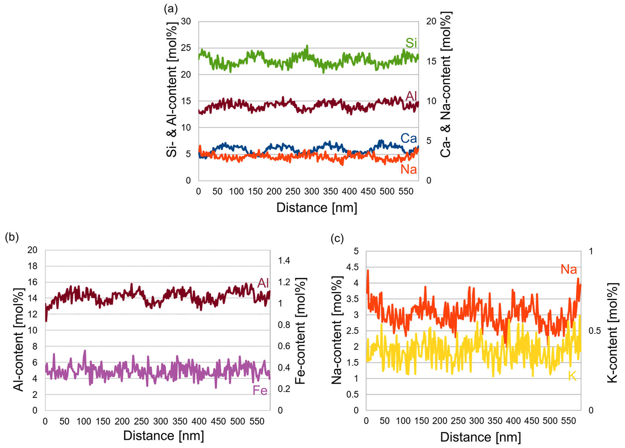
Figure 8EDS line scans with the element content (in mol%) plotted against distance in nanometers. (a) Si, Al, Ca and Na; (b) Al and Fe; (c) Na and K. In order to display the trend of each element, there are two y axes in each diagram.
4.3 Atomic scale investigations – HRTEM imaging
A high-resolution image (Fig. 9a) oriented in the direction [010] was recorded. In the fast Fourier transform (FFT), a* (a=8.2 Å) and c* (c=7.1 Å) can be seen (Fig. 9b). The angle between a* and c* is ∼ 64∘, which in real space equals the ∼ 116∘ of β. The high-resolution transmission electron microscopy (HRTEM) image was filtered with the diffraction spots of the labradorite cell with a doubled c axis, including the satellites that reflect the modulation vector. We applied a mask by using the 002 and the 200 reflections, and, in addition, one filter mask was created also including the satellite reflections. In Fig. 9b the filtered FFT is shown including the satellites. Please note that when unmodulated and modulated FFTs are compared, no significant changes were detected because the modulation vector is inclined to the [010] direction. In Fig. 9c, the labradorite structure oriented along [010] was superimposed on a magnified region of Fig. 9a, which agrees well with the high-resolution structure. Si and Al are shown in blue and are located on the bright positions. Ca and Na are shown in yellow and are positioned on the border of the dark areas. The FFT of the HRTEM image reveals additional maxima, which can be attributed to a modulation. The distance of these satellites indicate a period of 4.3 nm. In order to calculate the actual modulation of labradorite it is necessary to measure and reconstruct the labradorite diffraction space in three dimensions.
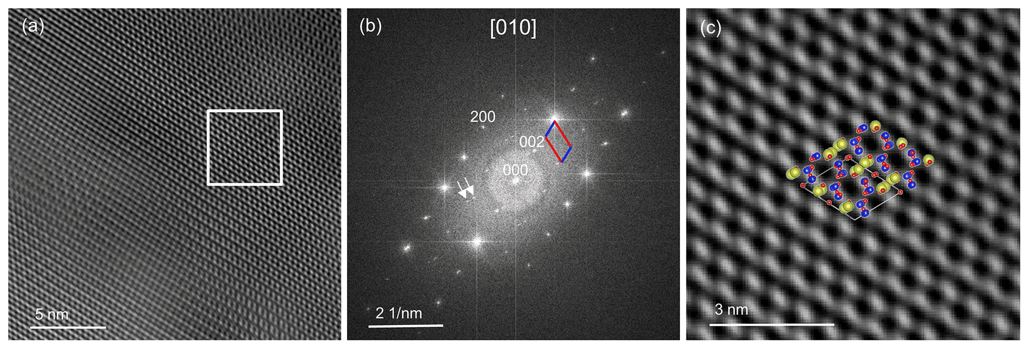
Figure 9(a) High-resolution TEM images of labradorite along the [010] direction. The intensity is modulating because of an increase in sample thickness throughout the image. The image is filtered with the cell with a doubled c axis from its FFT, which is displayed in (b). The a* and c* axis are shown in the FFT in red and blue, respectively. The white arrows indicate satellite reflections. (c) Magnified top-right area (boxed region) of the filtered HRTEM image from (a). The labradorite structure correlates well with the high-resolution structure. Si and Al are displayed in blue, Na and Ca in yellow, and O in red.
4.4 Average crystal structure solution – three-dimensional electron diffraction
For the acquisition of 3DED data using automated diffraction tomography (ADT) a lamella that extended into the thinned hole (Fig. 10) was selected. Since Ca-rich plagioclase is more stable up to higher temperatures than Na-rich plagioclase, the Ca-rich lamellae are more resistant to ion thinning. When only considering the Ca-rich lamellae in the EDS line scan (Fig. 7), the An content of the extending lamellae is around 60 % and thus higher than the concentration averaged over several lamellae (compare with Fig. 10).
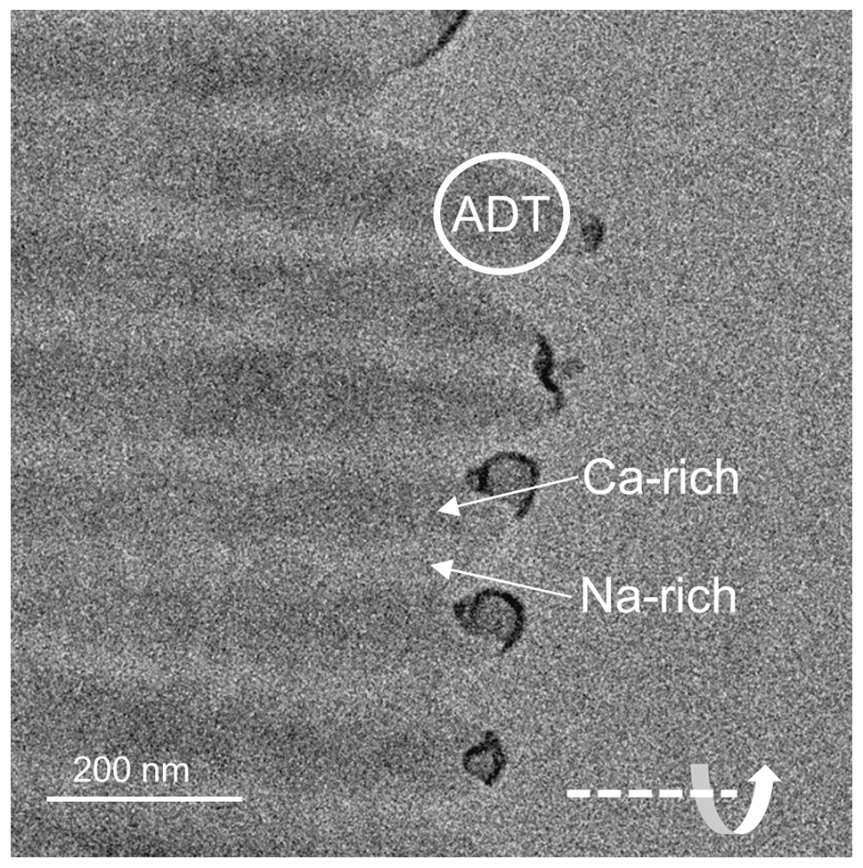
Figure 10TEM bright-field image of the lamellae. The thicker Ca-rich lamellae extend further into the thinned hole due to their higher resistance against ion thinning. The position where the ADT data set was taken is marked with a white circle. The horizontal tilt axis is shown in the bottom-right corner.
The data sets usually ranged from −60 to +60∘ and contained up to 121 frames recorded for tilt steps of 1∘. They were captured using a beam size of 150 nm, 0.5 s exposure time, a camera length of 1 m and a precession angle of 1∘. Out of 30 data sets, two sets (orientations 1 and 2 from the same lamella) with the best visibility of satellite reflections were chosen for further evaluation, structure solution and refinement. The analysis of the reconstructed three-dimensional reciprocal space delivered the following cell parameters: a=8.164(2) Å, b=12.898(3) Å, c=7.163(2) Å, α=94.28(3)∘, β=116.52(2)∘ and γ=89.47(2)∘. This cell is close to the unit cell of Jin et al. (2020), who worked on a comparable composition of An52 (Sample 7147A): a=8.1640(3) Å, b=12.8534(2) Å and c=14.2098(4) Å, respectively, 7.1049 Å for the single cell, and α=93.6187(11)∘, β=116.2531(15)∘ and γ=89.781(3)∘. The maximum deviation in cell axes and angles is below 1 %.
In Fig. 11 for the three main orientations, together with the main zones [100], [010] and [001], the derived cell parameters and the full reciprocal space viewed down c* are shown. The view down c* (Fig. 11d) exhibits only reflections with hkl: indicating a C-centered cell. Apart from these reflection conditions, also observable in the main zones [010] (h0l: h=2n) and [100] (0kl: k=2n), no additional extinctions were detected. This corresponds to the known space group (Wenk et al., 1980) describing all basic reflections.
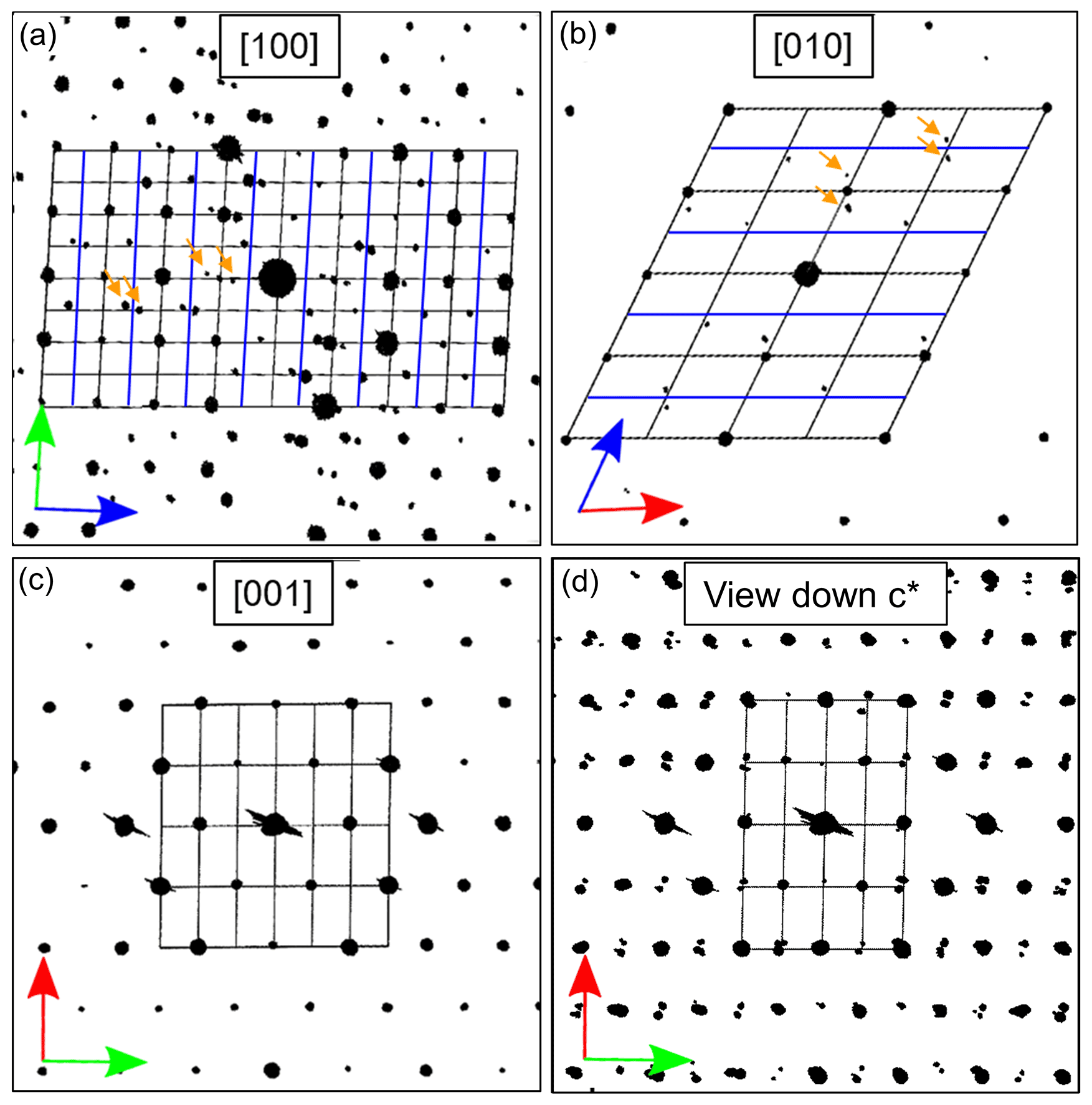
Figure 11Cut of three main zones and projection of the reconstructed ADT diffraction volume (unit cell of labradorite indicated with black lines, arrows in red = a* axis, green = b* axis and blue = c* axis, and blue lines indicate c-axis doubling). (a) [100], (b) [010], (c) [001] direction. (d) Projection of the reciprocal space along c* showing C-centering and satellite reflections. In (a) and (b) satellite reflections are indicated by orange arrows.
In addition, satellite reflections can be seen in the three-dimensional-reconstructed space (see orange arrows in Fig. 11a and b), which do not originate from the basic structure. However, these reflections are regularly arranged. As described in Fig. 1, f-satellite reflections define themselves around the a-reflections and e-satellite reflections around the position of absent b-reflections. The basic cell derived from the ADT diffraction volume cannot be used to describe the b-reflections in the structure; thus the c axis must be doubled (indicated by blue lines in Fig. 11a and b).
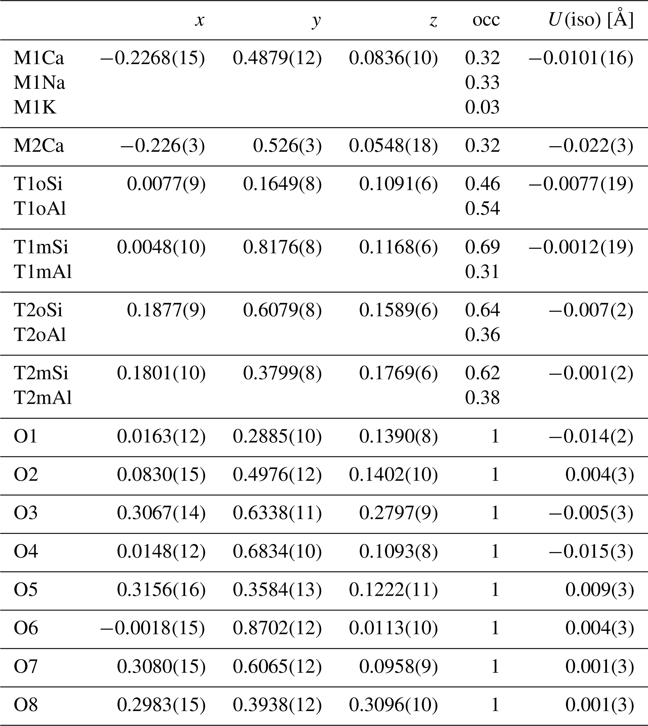
The electron diffraction data were extracted with the program PETS2 (Palatinus et al., 2019) for both the single cell without satellite reflections and the doubled cell including satellite reflections. In a first step, a structure solution without satellite reflections was performed in space group with Jana2006 (Petříček et al., 2014) using the composition derived from EDS measurements Na0.36Ca0.60K0.04Si2.4Al1.6O8 and Z=4, which led to a density of 2.72 g cm−3. The data sets reached a maximum completeness of 84.29 %, providing a sufficient coverage of the reciprocal space to solve the average structure of labradorite using the charge-flipping algorithm (Palatinus, 2013) of Superflip (Palatinus and Chapuis, 2007). For direct comparison with the crystal structure solved from X-ray radiation (Jin and Xu, 2017a), an origin shift of , , 0 had to be applied. Crystallographic details are given in Table 1. The structure consists of four Al and Si tetrahedra that are connected to each other in a framework. Additionally, there are two cation positions (M) in slightly irregular coordination polyhedra. A detailed figure of the structure with the respective names of all the atoms is given in S2. The highest potential found with an octahedral coordination was assigned to Ca, Na and K (M1). After refinement an additional potential was detected next to M1 and assigned to Ca (M2; occupancy of M1 + M2 = 1). The occupancies of the four tetrahedral positions containing Si and Al were calculated based on the average T–O distances of each tetrahedron. This was done following the equation developed by Kroll and Ribbe (1983), where
with nAn being the An content (0.60), 〈Ti−O〉 being the average individual distances of one tetrahedron, 〈〈T−O〉〉 defined as the grand mean tetrahedral distances, and k being a constant of ∼ 0.135 Å (Angel et al., 1990). The average individual distances of the tetrahedra can be found in Sect. S3. This results in an Al occupancy of 0.36, 0.54, 0.31 and 0.38 for T2o, T1o, T1m and T2m, respectively, and is in good agreement regarding the Ca and Na content. These occupancies were kept fixed during the refinement.
The kinematical least squares refinement converged with a weighted R value (wR(all)) of 31.04 %. The structure that resulted was reasonable; however, some atomic displacement factors were negative. A dynamical refinement based on the kinematical structure model resulted in a sample thickness of 528 and 870 Å for data from orientations 1 and 2, respectively, with an overall wR(all) of 10.49 %. All atom positions and occupancies are tabulated in Sects. S4 and S5. The refined occupancy of Ca in both of the M positions resulted in an overall Ca content of ∼ 0.64, which is close to the results derived from EDS measurements. At 4σ there is no residual electron potential left, so it can be assumed that all atomic positions are occupied satisfactorily. Some anisotropic displacement factors (ADPs) remained negative throughout the dynamical refinement. The atomic displacement factors of nearly all atoms (except O2) show an elongation along the b axis due to the missing diffraction information in the data sets. Nevertheless, the M2 position shows a very high ADP pointing in the direction of the M1 position, hinting at the modulation, which was not taken into account in the average structure solution based on major reflections.
Compared to the kinematical structure solution, the atom positions in the dynamical one differ slightly. The smallest displacement has T2o with a discrepancy of 0.0061 Å and the largest M1 with 0.1017 Å. The average difference of the two structures calculated with COMPSTRU of the Bilbao Crystallographic Server (de la Flor et al., 2016) is 0.0335 Å. Compared to the average labradorite structure of Jin and Xu (2017a), the smallest and largest displacements are also for the T2o with 0.006 Å and M1 position with 0.1796 Å. The average displacement is 0.032 Å. The bond lengths for T–O (expected to be 1.618 Å for Al, 1.596 Å for Si) and M–O (expected to be 2.336 Å for Na, 2.33 Å for Ca) are in a reasonable range (see Sect. S3 for all bond lengths). The maximum T–O distance is 1.697 Å for T1o–O8. The distance between M1 and M2 is 0.78 Å.
Table 1Crystallographic details concerning the labradorite structure and its refinement. The goodness of fit is abbreviated as GOF.
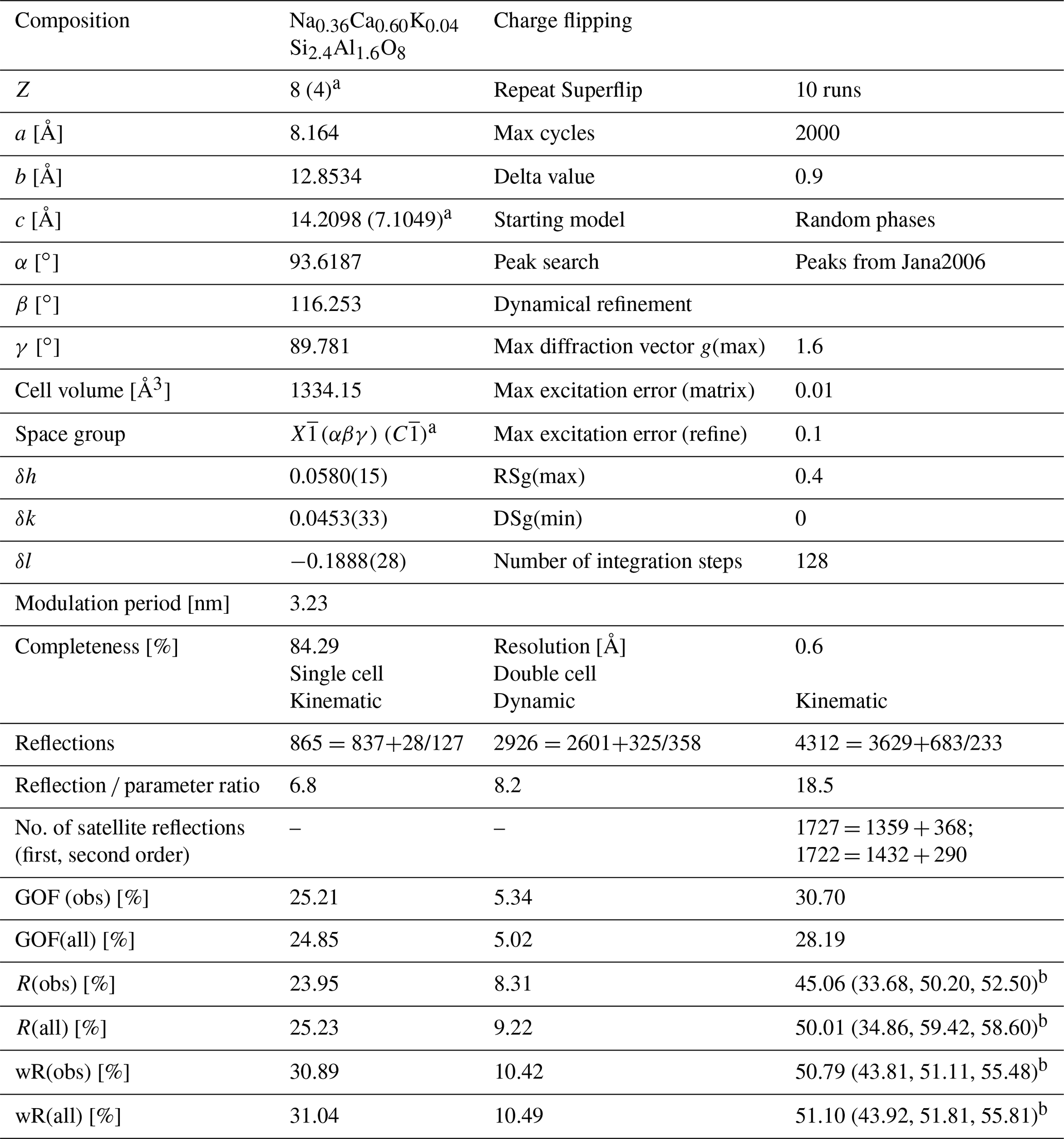
a Values in brackets are describing the single cell; b values in brackets are describing the values for main reflections, first-order satellite reflections and second-order satellite reflections.
4.5 Modulated crystal structure solution – three-dimensional electron diffraction
For a full description of the labradorite structure, incommensurate characteristics need to also be considered. Half of the distance between the e-reflections, which are found symmetrically around the absent b-reflections, equals the vector t (), resulting in a length of 6.46 nm. The distance between the second-order f-reflections and the a-reflections equals (3.23 nm). The modulation vectors of the e and f-reflections are parallel and describe a straight line connecting the a-reflection with both f and e-reflections (see dashed green line in Fig. 1). The angle of the t vector to the c* axis is 34∘. It lies approximately along (11–4). The vector t is 9.25 times longer than the cell vector in this direction (3.49 Å). Thus, it is not an integer multiple of the cell vector, confirming the incommensurate structure of labradorite. In order to incorporate e-reflections into the data set for structure solution, a double c axis of 14.2098 Å was used (see as well Fig. 11). Additionally, the modulation vector t needs to be applied in order to index first- and second-order satellite reflections found in the data set. This led to a special centering condition of ( 0), (0 0 ), ( 0 ) and required an expansion of the three-dimensional space to a three-plus-one-dimensional ((3 + 1)D) superspace. In this case, the space group was used. It is listed in Stokes et al. (2011) as 2.1.1.1, where X indicates a non-standard centering and triclinic point group. (αβγ) shows that the modulation vector has components along every main direction (δh, δk, δl as listed in Table 1). 0 indicates that no further translation is applied.
A kinematical refinement was performed based on this preliminary average crystal structure refined only on main reflections (see Sect. 4.4.), which resulted in a wR(all) of 51.10 %, split for main reflections and first- and second-order satellites into 43.92 %, 51.81 % and 55.81 %, respectively (for details see Table 1). For the structure refinement, the atomic displacement factors were kept isotropic, and harmonic position modulations up to the second order were used for each atom. Additionally, second-order occupancy modulations were applied to the M and T sites. For a detailed listing of all modulation waves, see Sects. S6 and S7.
The resulting average structure of labradorite is shown in Fig. 12, and its average atomic positions are displayed in Table 2. This structure agrees well with the structure solution of the single cell with a doubled c axis. The smallest displacement appears for T2o with 0.0239 Å, and the biggest difference in position has M2 with 0.1338 Å. The average displacement is 0.0532 Å (calculated with COMPSTRU of the Bilbao Crystallographic Server; de la Flor et al., 2016). Compared to the modulated labradorite structure of Jin and Xu (2017a), the smallest difference in the atom position is 0.016 Å for T1m and the largest 0.0762 Å and 0.0747 Å for O4 and M2, respectively. The average displacement is 0.0455 Å. The average T–O bond distances are in good agreement with expected values; however, the range of a single bond length caused by the modulation is rather large. The maximum ranges for each tetrahedron are T1o–O1 (1.27–1.99 Å), T2o–O3 (1.35–1.83 Å), T1m–O4 (1.43–2.05 Å), T2m–O5 (1.32–1.96 Å). All bond lengths are tabulated in Sect. S8.
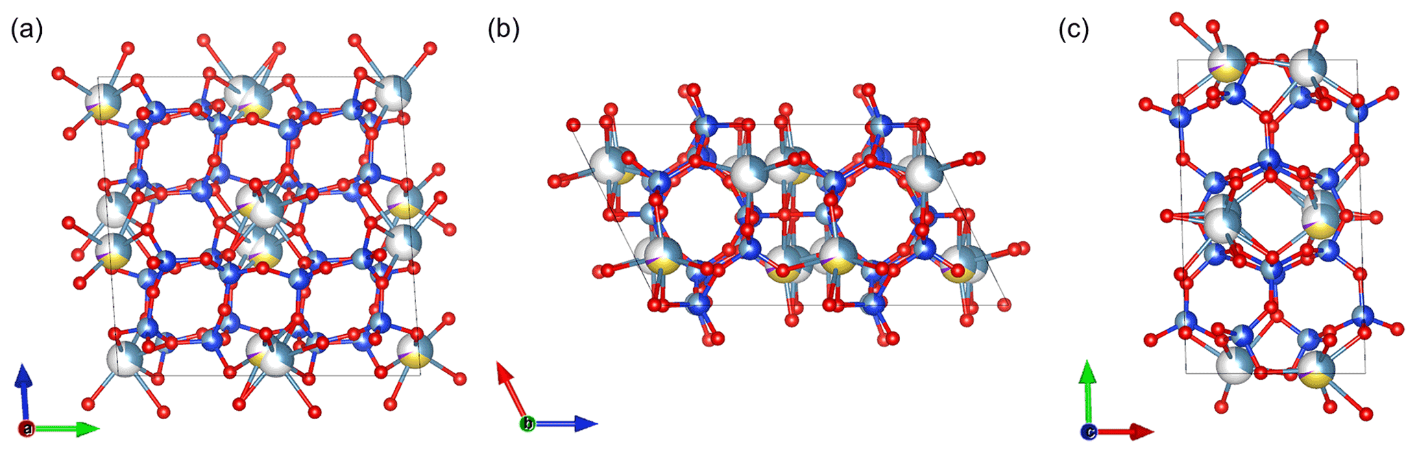
Figure 12Average structure of labradorite viewed along (a) [100], (b) [010] and (c) [001]. Ca is displayed in light blue, Na in yellow, K in purple, Si in dark blue, Al in grey and O in red.
Table 2Average positions of the atoms in the modulated labradorite structure (xyz) with occupancy (occ) and isotropic atomic displacement factors (U(iso)).
In order to image the modulation from (3+1)D space, the structure of labradorite is approximated over several cells (4xa, 4xb, 4xc). Figure 13a shows the structure along [1–10], which is approximately perpendicular to the modulation vector. Only one layer of M positions was cut out parallel to [1–10] to illustrate the change in position of the atoms, as well as the occupancy of the M and T sites. The M positions modulate between Na-rich–Ca-poor and Na-poor–Ca-rich compositions. This can further be illustrated by plotting the occupancy of the M position versus the modulation (Fig. 13b). The Na occupancy of the M1 position was fixed to modulate identically to the K occupancy and complementary to the Ca occupancy of M2. The additional coupling of the ratio at each position according to Ca occupancy has been taken into account but is not shown in Fig. 13b. Within one modulation period, the M1 site changes between a preferred Ca and Na occupancy. The Ca of the M2 position reaches its maximum occupancies at around the same t as that of the M1 position.

Figure 13(a) Modulated structure of labradorite displayed over four cells along the a, b and c axes. Viewing direction along [1–10] providing the view perpendicular to the modulation vector [11–4] (black line) and the modulation direction (black arrow). Only one layer of the M positions is displayed. (b) Modulation of the occupancy of the M site versus t. M1 is displayed in green and M2 in cyan.
In Fig. 14 de Wolff sections, displaying the position modulation, are shown for the two M positions, as well as the T2o tetrahedron with its adjacent oxygen (O2, O3, O4, O7). In (3+1)D superspace the four axes are assigned to the three main axes of the cell (x1–3) and the modulation vector (x4). The de Wolff sections show the observed electron potential for a selected atom in black and the position modulation of this atom along the modulation vector in color. In this case, the sections were selected exemplarily for a variable x4 and x3, with x1 and x2 being fixed. For de Wolff sections of all three main directions for the M positions, see Sect. S9. The harmonic modulations up to the second order improve the position of each atom and allow them to fit their observed electron potential nicely. The position modulation of the M sites influence the tetrahedra and their adjacent oxygen, which causes them to modulate similarly.

Figure 14De Wolff sections for (a) both M positions and (b) T2o and its adjacent oxygen: (c) O2, (d) O3, (e) O4 and (f) O7. In the graphs, the position modulation of each atom is plotted over their observed electron potential in the x4 (modulation direction) versus x3 (c axis) plane for a given x1 (a axis) and x2 (b axis) value. The M2 position is displayed in cyan, M1 in green, T2o in blue and O in red.
In order to compare the properties of labradorite with the results of Miúra et al. (1975), the thickness of the both lamellae must be taken into account. According to Eq. (1), a total thickness of 193(2) nm results in a wavelength of 3.105⋅193(2) nm − 2.1178 nm = 597(6) nm, which means that the labradorescence color should be yellow. This agrees with the actual labradorescence color. According to Eq. (2), this should correspond to an An content of mol% = 53.45(18) mol%, which also matches the An content of about 53.4 % measured here. The Or content of 5.1 mol% measured here agrees with the statement of Nissen et al. (1973) that all labradorites exhibiting schiller have an Or content of at least 2 mol%.
The labradorite lamellae are tilted approximately 11∘ away from the b axis. A majority of the lamellae studied in the literature to date lie at ∼ 14∘ to the b axis (Raman and Jayaraman, 1950; Lord Rayleigh, 1923), but other angles occur as well (9–21∘; Bøggild, 1924). It follows that the position of these lamellae is similar to the usual orientation.
To describe the satellite reflections of the labradorite structure, the c axis must be doubled. The modulation vector t was compared with experiments from Jin et al. (2020). For the respective corresponding graphs, see Sect. S10. All values of t lie within the expected range for a labradorite with approximately 53 % An content, being also consistent with the length of the satellite vector of 3.23 nm. After the nomenclature of Jin et al. (2020) this labradorite would be described as an eα-labradorite. This classification was based on the modulation period of t, in which eα has a shorter period than eβ. The δl value is more in the eβ range; however, this could arise from slight inaccuracies in the modulation vector measurement. eα appears only when the structure was reset by going through an intermediate stage. There are two possible ways of achieving this. In this case, the eα-structure was achieved by forming lamellae. Another way would be to form the centered structure, which is not possible for a labradorite with an An content of ∼ 53 mol%.
The structure solution was performed on a single Ca-rich lamella. The averaged An content of the Ca-rich lamellae of 60 % agrees relatively well with the refined An content of the structure solution of 64 %. The tetrahedral positions were not occupied based solely on the EDS results. This would assign all tetrahedral positions an equal ratio, which is not the case for a labradorite. Instead, the tetrahedral occupancies were calculated based on the T–O bond lengths of the individual tetrahedra. This served as a guide because the errors in the bond lengths are around 0.5 % with electron diffraction, and thus the occupancies cannot be calculated as accurately as with X-ray diffraction. However, the occupancies of the tetrahedral positions calculated with this method (Al(T1o) = 54 % (57 %), Al(T2o) = 36 % (29 %), Al(T1m) = 31 % (31 %), Al(T2m) = 38 % (34 %)) are close to those defined in the X-ray structure of Jin and Xu (2017a) (results in brackets) used for crystal structure solution.
The dynamical refinement of the average structure agrees well with the already existing structures solved by X-ray diffraction (Jin and Xu, 2017a). The atomic positions and distances are in reasonable agreement with each other, with larger errors calculated for electron diffraction data.
Since the cell parameters cannot be changed significantly for each lamella, the only way of balancing the different compositions is to introduce a modulation into the structure. The modulation is mainly caused by the M positions. Ca moves further away from its original position than Na (Xu et al., 2016). However, their movements also influence the other atoms in the cell. This causes the oxygen atoms, which are located near the M positions, to modulate strongly as well. The modulation of the occupancy of the M positions is also accompanied by a modulation of the tetrahedral occupancies (Kitamura and Morimoto, 1977). The replacement of Na by Ca in the M1 site can be seen as an implementation of internal stress, since Ca is bigger than Na. In the labradorite framework, a change in the T–O–T angles compensates for the applied stress, which leads to a shortening of the crankshaft chains (Angel et al., 1988).
This study discusses the various structural features present in labradorite from the original piece through several orders of magnitude down to the atomic scale, allowing a variety of structural features to be seamlessly investigated. The labradorite samples selected by polarized light microscopy were prepared as ion-milled samples in three different orientations and investigated by TEM and STEM imaging, providing a direct relation to the features visible in the light microscope. Twins, lamellae and additional domains with e-fringes were recognizable. The labradorite is strongly twinned by albite – as well as pericline – twin laws. Because of the difference in the direction of b* compared to the matrix, pericline twins show a slightly different orientation of the lamellae and are thus displaying labradorescence at different glancing angles, θ. The lamellae, which are the cause of the labradorescence, are alternating between Ca-rich and Na-rich as derived from EDS line scans. The size of the measured lamellae averaged 129 nm for the Ca-rich lamellae and 64 nm for the Na-rich lamellae. The ratio influences the overall thickness of the lamellae pair, thus also influencing the color of labradorescence. The average composition of this labradorite is An53.4Ab41.5Or5.1. The reflective wavelength obtained by applying the equations of Miúra et al. (1975) gives a labradorescence color of yellow, which agrees well with the actual color of the samples taken. The calculated An content is identical to the measured An content of about 53.4 %.
The application of high-resolution TEM in principle reveals structural details; however, we were not able to visualize the modulation of the atomic position (or occupancy) except for the satellite reflections in the corresponding FFT. In addition, using 3DED for the analysis of a single Ca-rich lamella of ∼ 120 nm width delivered electron diffraction data sets suitable for “ab initio” crystal structure analysis of both the average crystal structure of labradorite and its complex incommensurate modulation. The modulation is caused by the inability to reach a Ca–Na-ordered state of the system, leading to alternating Ca-rich and Ca-poor lamellae with slight chemical and structural differences. The modulation vector t could be determined as being with a period of 3.23 nm. This causes e-fringes, which can be seen in domains inside the Ca-rich lamellae and are parallel to (11–4) (Hashimoto et al., 1976; Korekawa et al., 1979). The modulation occurs due to the incommensurate structure of the labradorite but has no effect on the labradorescence.
The investigation of the incommensurate crystal structure of labradorite allowed for the direct comparison of the structure derived by X-ray single crystal structure analysis (Jin and Xu, 2017a) with the structure based on electron diffraction data. While X-ray diffraction data were collected from a micrometer-sized sample averaging over a large number of Ca-rich and Ca-poor lamellae, electron diffraction data originate from one single Ca-rich lamella in the nanometer regime. In general, electron diffraction delivers sharper-defined density maps due to the strong interaction of the electron beam with the atomic core. Nevertheless, the distribution along the modulation vector differs and is more clearly defined for 3DED data, which may be caused by the restriction to a single Ca-rich lamella (compare de Wolff sections shown in Sect. S9 to the ones of Jin and Xu, 2017a). The generally small deviation of the average structures between the X-ray single crystal and three-dimensional electron diffraction approaches demonstrates again the potential of 3DED to solve and reliably refine complex crystal structures with low symmetry.
Data for the structure solution of the average and incommensurate structures are available in the Supplement.
The supplement related to this article is available online at: https://doi.org/10.5194/ejm-34-393-2022-supplement.
EG carried out the sample preparation, analyzed the samples with electron microscopy, evaluated the results and prepared the manuscript. HJK and UK were involved in project planning, supervised the project and reviewed the manuscript. All authors read and approved the final manuscript.
The contact author has declared that none of the authors has any competing interests.
Publisher's note: Copernicus Publications remains neutral with regard to jurisdictional claims in published maps and institutional affiliations.
The authors are thankful to Sergi Plana-Ruiz for his help and fruitful discussions regarding the ADT data acquisition.
This research has been supported by the Bundesministerium für Wirtschaft und Energie (grant no. 0324244A).
This paper was edited by Massimo Nespolo and reviewed by Mario Tribaudino and one anonymous referee.
Angel, R. J., Hazen, R. M., McCormick, T. C., Prewitt, C. T., and Smyth, J., R.: Comparative Compressibility of End-Member Feldspars, Phys. Chem. Miner., 15, 313–318, https://doi.org/10.1007/BF00311034, 1988.
Angel, R. J., Carpenter, M. A., and Finger, L. W.: Structural variation associated with compositional variation and order-disorder behavior in anorthite-rich feldspars, Am. Mineral., 75, 150–162, 1990.
Benna, P., Tribaudino, M., and Bruno, E.: Al-Si Ordering in Sr-Feldspar SrAl2Si2O8: IR, TEM and Single-Crystal XRD Evidences, Phys. Chem. Miner., 22, 343–350, 1995.
Bøggild, O. B.: On the labradorization of the feldspars, Det Kongelige Danske Videnskabernes Selskab Mathematisk-Fysiske Meddelelser, 6, 1–81, 1924.
Bolton, H. C., Bursill, L. A., McLaren, A. C., and Turner, R. G.: On the origin of the colour of labradorite, Phys. Status Solidi C, 18, 221–230, https://doi.org/10.1002/pssb.19660180123, 1966.
Boullay, P., Palatinus, L., and Barrier, N.: Precession electron tomography for solving complex modulated structures: the case of Bi5Nb3O15, Inorg. Chem., 52, 6127–6135, https://doi.org/10.1021/ic400529s, 2013.
Burla, M. C., Caliandro, R., Carrozzini, B., Cascarano, G. L., Cuocci, C., Giacovazzo, C., Mallamo, M. , Mazzone, A., and Polidori, G.: Crystal structure determination and refinement via SIR2014, J. Appl. Crystallogr., 48, 306–309, https://doi.org/10.1107/S1600576715001132, 2015.
Carpenter, M. A.: Experimental delineation of the “e” I-1 and “e” C-1 transformations in intermediate plagioclase feldspars, Phys. Chem. Miner., 13, 119–139, https://doi.org/10.1007/BF00311902, 1986.
Chao, S. H. and Taylor, W. H.: Isomorphous replacement and superlattice structures in the plagioclase feldspars, P. R. Soc. Lond., 176, 76–87, https://doi.org/10.1098/rspa.1940.0079, 1940.
de la Flor, D., Orobengoa, D., Tasci, E., Perez-Malto, J. M., and Aroyo, M. I.: Comparison of structures applying the tools available at the Bilbao Crystallographic Server, J. Appl. Crystallogr., 49, 653–664, https://doi.org/10.1107/S1600576716002569, 2016.
ESRI: ArcGIS Desktop: Release 10, Environmental Systems Research Institute, Redlands, CA, 2011.
Hashimoto, H., Nissen, H. U., Ono, A., Kumao, A., Endoh, H., and Woensdregt, C. F.: High-resolution microscopy of labradorite feldspar, in: Electron microscopy in mineralogy, edited by: Wenk, H. R., Springer Verlag, New York, United States, 332–344, ISBN 9783642661969, 1976.
Henn, U., Millisenda, C. C., and Stephan T. (Eds.): Gemmological Tables for the identification of gemstones, synthetic stones, artificial products and imitations, German Gemological Association, ISBN 9783000648564, 2020.
Hoshi, T., Tagai, T., and Suzuki, M.: Investigations on Boggild intergrowth of intermediate plagioclase by high resolution transmission electron microscopy, Z. Kristallogr., 211, 879–883, https://doi.org/10.1524/zkri.1996.211.12.879, 1996.
Jin, S. and Xu, H.: Solved: The enigma of labradorite feldspar with incommensurately modulated structure, Am. Mineral., 102, 21–32, https://doi.org/10.2138/am-2017-5807, 2017a.
Jin, S. and Xu, H.: Investigations of the phase relations among e1, e2 and C-1 structures of Na-rich plagioclase feldspars: a single-crystal X-ray diffraction study, Acta Crystallogr. B, 73, 992–1006, https://doi.org/10.1107/S2052520617010976, 2017b.
Jin, S., Xu, H., Wang, X., Jacobs, R., and Morgan, D.: The incommensurately modulated structures of low-temperature labradorite feldspars: a single-crystal X-ray and neutron diffraction study, Acta Crystallogr. B, 76, 93–107, https://doi.org/10.1107/S2052520619017128, 2020.
Kalning, M., Dorna, V., Burandt, B., Press, W., Kek, S., and Boysen, H.: High-Order Supersatellite Reflections in Labradorite. A Synchrotron X-ray Diffraction Study, Acta Crystallogr. A, 53, 632–642, https://doi.org/10.1107/S010876739700500X, 1997.
Kitamura, M. and Morimoto, N.: The superstructure of plagioclase feldspars. A modulated coherent structure of the e-plagioclase, Phys. Chem. Miner., 1, 199–212, https://doi.org/10.1007/bf00307318, 1977.
Kolb, U., Shankland, K., Meshi, L., Avilov, A., and David, W. I. F. (Eds.): Uniting Electron Crystallography and Powder Diffraction, Springer, Dodrecht, the Netherlands, ISBN 9789400755802, 2012.
Korekawa, M., Horst, W., Tagai, T., Joswig, W., and Wenk, H. R.: Structure determination of plagioclase (labradorite): I. Al/Si distribution in an An66 (neutron diffraction): II. Superstructure of An54 (X-ray diffraction), AIP Conf. Proc., 53, 311–313, https://doi.org/10.1063/1.31844, 1979.
Kroll, H. and Ribbe, P. H.: Lattice parameters, composition and Al,Si order in alkali feldspars, in: Feldspar Mineralogy, edited by: Ribbe, P. H., Mineralogical Society of America, Cantilly, Virginia, 57–100, https://doi.org/10.1515/9781501508547-008, 1983.
Lanza, A. E., Gemmi, M., Bindi, L., Mugnaioli, E., and Paar, W. H.: Daliranite, PbHgAs2S5: determination of the incommensurately modulated structure and revision of the chemical formula, Acta Crystallogr. B, 75, 711–716, https://doi.org/10.1107/S2052520619007340, 2019.
Lord Rayleigh: Studies of Iridescent Colour and the Structure Producing it. III. The Colours of Labrador Felspar, P. R. Soc. London, 103, 34–45, http://www.jstor.org/stable/94093 (last access: 14 September 2022), 1923.
Makada, R., Sato, M., Ushioda, M., Tamura, Y., and Yamamoto S.: Variation of Iron Species in Plagioclase Crystals by X-ray Absorption Fine Structure Analysis, Geochem. Geophy. Geosy., 20, 5319–5333, https://doi.org/10.1029/2018GC008131, 2019.
Miúra, Y.: Color zoning in labradorite, Mineralogical Journal, 9, 91–105, 1978.
Miúra, Y., Tomisaka, T., and Kato, T.: Labradorescence and the ideal behaviour of thicknesses of alternate lamellae in the Boggild intergrowth, Mineralogical Journal, 7, 526–541, https://doi.org/10.2465/minerj1953.7.526, 1975.
Nakajima, Y., Morimoto, N., and Kitamura, M.: The superstructure of plagioclase feldspars. Electron microscopic study of anorthite and labradorite, Phys. Chem. Miner., 1, 213–225, https://doi.org/10.1007/BF00307319, 1977.
Momma, K. and Izumi, F.: VESTA 3 for three-dimensional visualization of crystal, volumetric and morphology data, J. Appl. Crystallogr., 44, 1272–1276, https://doi.org/10.1107/S0021889811038970, 2011.
Németh, P., Tribaudino, M., Bruno, E., and Buseck, P. R.: TEM investigation of Ca-rich plagioclase: Structural fluctuations related to the I-1 – P-1 phase transition, Am. Mineral., 92, 1080–1086, 2007.
Nissen, H. U.: End member compositions of the labradorite exsolution, Naturwissenschaften, 58, 454–454, https://doi.org/10.1007/BF00624619, 1971.
Nissen, H. U., Champness, P. E., Cliff, G., and Lorimer, G. W.: Chemical evidence for exsolution in a labradorite, Nature Physical Science, 245, 135–137, https://doi.org/10.1038/physci245135a0, 1973.
Okrusch, M. and Matthes, S. (Eds.): Mineralogie: Eine Einführung in die spezielle Mineralogie, Petrologie und Lagerstättenkunde, Springer, Berlin, Heidelberg, Germany, ISBN 9783662087688, 2013.
Olsen, A.: Lattice parameter determination of exsolution structures in labradorite feldspars, Acta Crystallogr. A, 33, 706–712, https://doi.org/10.1107/S056773947700182X, 1977.
Palatinus, L.: The Charge-Flipping Algorithm in Crystallography, Acta Crystallogr. B, 69, 1–16, https://doi.org/10.1107/S2052519212051366, 2013.
Palatinus, L. and Chapuis, G.: SUPERFLIP – a computer program for the solution of crystal structures by charge flipping in arbitrary dimensions, J. Appl. Crystallogr., 40, 786–790, https://doi.org/10.1107/S0021889807029238, 2007.
Palatinus, L., Klementová, M., Dřínek, V., Jarošová, M., and Petříček, V.: An incommensurately modulated structure of η′-Phase of Cu3−xSi determined by quantitative electron diffraction tomography, Inorg. Chem., 50, 3743–3751, https://doi.org/10.1021/ic200102z, 2011.
Palatinus, L., Brázda, P., Jelínek, M., Hrdá, J., Steciuk, G., and Klementová, M.: Specifics of the data processing of precession electron diffraction tomography data and their implementation in the program PETS2.0, Acta Crystallogr. B, 75, 512–522, https://doi.org/10.1107/S2052520619007534, 2019.
Petříček, V., Dušek, M., and Palatinus, L.: Crystallographic Computing System JANA2006: General features, Z. Kristallogr., 229, 345–352, https://doi.org/10.1515/zkri-2014-1737, 2014.
Plana-Ruiz, S.: The Modulated Structure of Belite, in: Development & Implementation of an Electron Diffraction Approach for Crystal Structure Analysis, PhD thesis, Darmstadt, Barcelona, 177–200, 2020.
Plana-Ruiz, S., Krysiak, Y., Portillo, J., Alig, E., Estradé, S., Peiró, F., and Kolb, U.: Fast-ADT: A fast and automated electron diffraction tomography setup for structure determination and refinement, Ultramicroscopy, 211, 112951, https://doi.org/10.1016/j.ultramic.2020.112951, 2020.
Putnis, A. (Ed.): Introduction to mineral sciences, Cambridge University Press, Cambridge, England, https://doi.org/10.1017/CBO9781139170383, 2001.
Raman, C. V. and Jayaraman, A.: The structure of labradorite and the origin of its iridescence, P. Indian Acad. Sci. A, 32, 1–21, https://doi.org/10.1007/BF03172469, 1950.
Smith, J. V. (Ed.): Feldspar minerals – 2. Chemical and textural properties, Springer, Berlin, Heidelberg, Germany, ISBN 9783642657436, 1974.
Smith, J. V. and Brown, W. L. (Eds.): Feldspar Minerals – 1. Crystal Structure, physical, chemical and microtextural properties, Springer, Berlin, Heidelberg, Germany, 1988.
Steciuk, G., Boullay, P., Pautrat, A., Barrier, N., Caignaert, V., and Palatinus, L.: Unusual relaxor ferroelectric behavior in stairlike aurivillius phases, Inorg. Chem., 55, 8881–8891, https://doi.org/10.1021/acs.inorgchem.6b01373, 2016.
Stokes, H. T., Campbell, B. J., and van Smaalen, S.: Generation of (3+d)-dimensional superspace groups for describing the symmetry of modulated crystalline structures, Acta Crystallogr. A, 67, 45–55, https://doi.org/10.1107/S0108767310042297, 2011.
Wenk, H. R., Joswig, W., Tagai, T., Korekawa, M., and Smith, B. K.: The average structure of An 62–66 labradorite, Am. Mineral., 65, 81–95, 1980.
Xu, H., Jin, S., and Noll, B. C.: Incommensurate density modulation in a Na-rich plagioclase feldspar: Z -contrast imaging and single-crystal X-ray diffraction study, Acta Crystallogr. B, 72, 904–915, https://doi.org/10.1107/S205252061601578X, 2016.
Zuo, J. M. and Spence, J. C. H. (Eds.): Advanced Transmission Electron Microscopy – Imaging and Nanoscience, Springer, New York, United States, https://doi.org/10.1007/978-1-4939-6607-3, 2017.